> ## Documentation Index
> Fetch the complete documentation index at: https://docs.cosmosid.com/llms.txt
> Use this file to discover all available pages before exploring further.
# Beta diversity on Cosmos-Hub 2.0
> Run beta-diversity analysis in Cosmos-Hub 2.0: the plots and tables it produces, how to read them, and the parameters that shape them.
This page covers how beta-diversity analysis works on Cosmos-Hub 2.0: the outputs it produces, how to read them, and the parameters you can tune. For the theory behind beta diversity and the ordination methods, see the [Beta diversity overview](/analysis/beta-diversity/overview).
# Module output and customization
* **Beta-diversity ordination plot(s):** one ordination plot for each method currently available on Cosmos-Hub 2.0 (PCoA, MDS, t-SNE, and UMAP).
* **PCoA scree plot:** a PCoA-specific plot showing the proportion of distance variation captured by each PCoA axis.
* **Beta-diversity Statistical testing (Permanova and Anosim):** a heatmap showing statistical support for differences between the groups defined by the grouping variable, one cell per pairwise comparison.
* **Statistical output tables (5):** the data behind the PCoA ordination and scree plot, plus the PERMANOVA and ANOSIM results for the overall and pairwise group comparisons.
## Beta-diversity ordination plot(s)
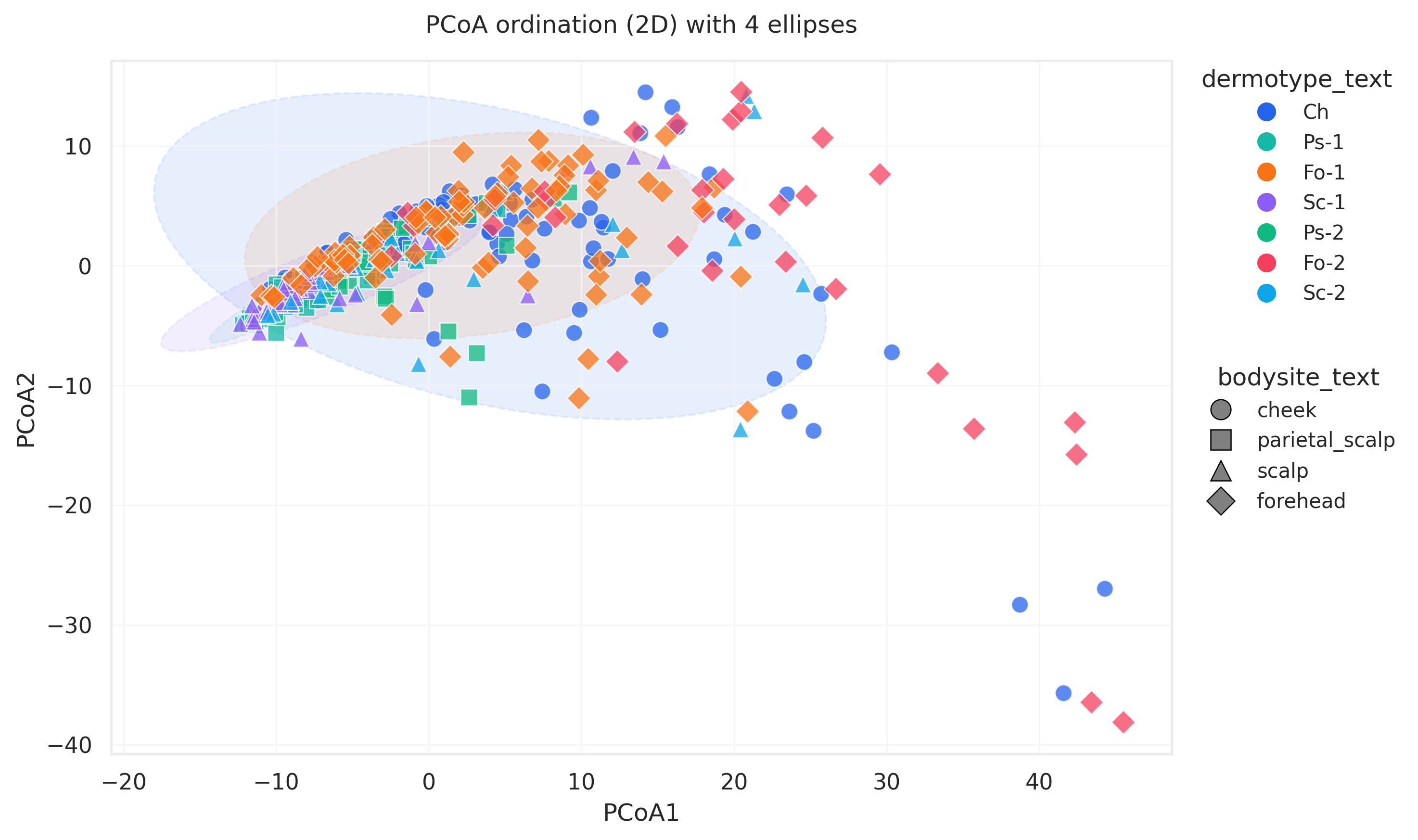 The ordination plot maps how microbial communities relate to one another across samples, based on how similar or different their compositions are.
* Each point represents one sample: the **distance separating two points** in the ordination plot is proportional to how different their microbial feature profiles are. When working with taxonomic profiles, distance tells you how similar their microbial communities are. When looking at functional profiles, it tells you how similar their functional profiles are.
The ordination plot maps how microbial communities relate to one another across samples, based on how similar or different their compositions are.
* Each point represents one sample: the **distance separating two points** in the ordination plot is proportional to how different their microbial feature profiles are. When working with taxonomic profiles, distance tells you how similar their microbial communities are. When looking at functional profiles, it tells you how similar their functional profiles are.
**1. Choose how to measure sample distances.**
Choose the method used to calculate the sample-to-sample pairwise distance matrix from the [**Beta-diversity metric**](#beta-diversity-metric) dropdown. This choice is important, as it actively changes how [the distance matrix](/DAP_docs/betadiversity-overview) used by the ordination methods for plotting is generated. Different beta-diversity metrics can lead to profoundly different ordination plots.
A few of the most popular metrics include:
* **Bray-Curtis**: for relative-abundance data, when you want differences in composition to be weighted by how abundant each taxon is. It is a popular, intuitive default.
* **Jaccard**: specific for presence/absence data. Useful when you care about which taxa are shared or not shared, regardless of their abundance.
* **Aitchison**: when you want to keep into account the compositional nature of sequencing data. Because sequencing measures relative, not absolute, abundances, an apparent rise in one taxon can just reflect a drop in another, which can create spurious patterns.
**How Aitchison works?** The Aitchison metric addresses compositionality by comparing samples using log-ratios between features. It first applies a CLR (centered log-ratio) transformation, where each feature in a sample is divided by a per-sample reference value and then log-transformed. When Aitchison is selected as distance metric from the parameter, the [**Centroid Method**](https://docs.cosmosid.com/#centroid-method) lets you set this per-sample reference value. You can choose between:
* `Mean`: the geometric mean of the sample (the standard CLR choice). Best when the data is fairly clean.
* `Median`: more robust to outliers and noisy low-abundance taxa, often useful for sparse data.
### 2. Customize the ordination plot
Once distances are computed, these parameters control how the plot is built and annotated:
* From your categorical metadata variables, choose one of interest from the [**Grouping Variable**](#grouping-variable) parameter dropdown. Data points in the ordination plots are assigned different colors depending on which group of that variable they belong to. This is the main way to visually inspect whether the variable you chose (treatment, body site, and so on) displays any pattern in the community structure.
Choice of the Grouping Variable governs between which groups PERMANOVA/ANOSIM testing is done.
* Overlay a second categorical variable as point shape using the [**Shape Variable**](#shape-variable) parameter. This is useful to keep track of another categorical variable (for example, Treatment encoded as the Grouping variable + Timepoint encoded as the Shape variable).
* Choose to display the ordination plot in 2D or 3D: change the [**Number of Components**](#number-of-components) parameter. A 2D ordination plot is usually the best choice to maintain readability of the plot, but a 3D plot can be useful when the first two components do not capture enough of the variation, so an important separation between groups stays hidden in 2D but becomes visible once a third axis is added.
* The [**Max ellipses**](#max-ellipses) and [**Confidence level**](#confidence-level) parameters control the group ellipses drawn on the plot, which summarize where each group of samples sits and how spread out it is.
* [**Drop samples with missing grouping metadata**](#drop-samples-with-missing-grouping-metadata) removes samples that have no value for the grouping variable, keeping the plot and the comparison clean.
Keeping them can instead be useful to get a sense of where an unlabeled sample falls, for example whether it sits near a known group.
#### **Why it's useful**
* **Explore overall similarity:** close samples have similar communities; distant samples differ.
* **Assess whether your metadata explains community structure:** color samples by a variable (treatment, disease status, body site, and so on) and check whether it lines up with visible patterns. If the groups are **mixed**, that variable may not explain much of the variation; if they **cluster or separate**, it may be associated with community differences, but first rule out study-design or technical variables (batch, cohort, sampling site).
* **Spot batch or technical effects:** if samples cluster by sequencing batch, study site, run, extraction method, processing date, or cohort, consider this before reading the pattern as biology.
* **Detect outlier or suspicious samples:** samples expected to be similar (replicates, or longitudinal samples from one subject) should sit close together. If one clusters with an unrelated subject, it may be a true biological shift, or a sample swap, label mismatch, contamination, or processing issue worth checking.
### 3. Statistical testing
The ordination plot gives a visual cue of whether your grouping variable drives overall community differences. Statistical testing confirms whether that visual clustering is supported by the data.
The Beta-diversity analysis module lets you test whether the cluster separation between all group pairs of the grouping variable you chose is significant, by performing pairwise **PERMANOVA** and **ANOSIM** tests.
The two main parameters controlling the testing are:
* The [**Grouping Variable**](#grouping-variable) defines the groups being compared. It is the same variable you used to color the plot, which is why the visual pattern and the statistical result line up.
* The [**Number of permutations**](#number-of-permutations) sets how finely the null distribution is estimated. More permutations give a more precise p-value, at the cost of longer run time.
The result of statistical testing is summarized by the Permanova/Anosim heatmap:
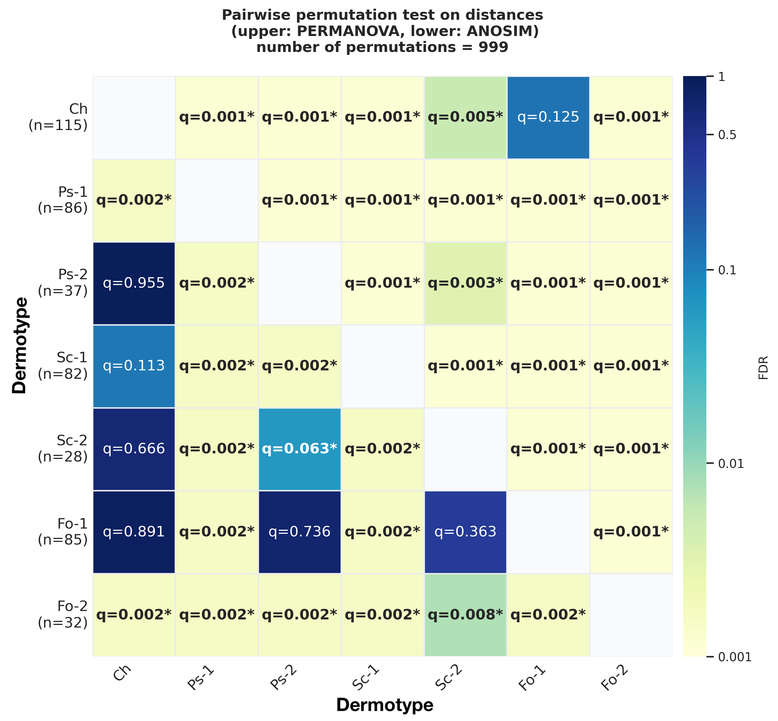 The heatmap answers this by running a separate test for every pair of groups. Each cell is the **FDR-adjusted q-value** for one pairwise comparison, and lower values mean stronger evidence that those two groups differ in composition.
The q-value is a p-value that has been adjusted for multiple testing. Running many pairwise comparisons inflates the chance of a false positive, so the adjustment (false discovery rate, or FDR) corrects for the number of comparisons, keeping the results trustworthy when you read the whole heatmap at once.
**What are PERMANOVA and ANOSIM?** Both test whether samples from the same group are more similar to each other than to samples from other groups, that is, whether your grouping variable separates the data better than random chance would.
* **PERMANOVA** tests whether the grouping variable explains the differences in the distance matrix, using a pseudo-F statistic (similar in spirit to ANOVA, but on distances between samples rather than on a single measured variable). It is the common choice for whether overall composition differs between groups.
* **ANOSIM** also tests group separation, but by ranking distances and comparing within-group to between-group distances. Its statistic **R** ranges from about −1 to 1, with values near 1 indicating stronger separation.
## PCoA scree plot
The heatmap answers this by running a separate test for every pair of groups. Each cell is the **FDR-adjusted q-value** for one pairwise comparison, and lower values mean stronger evidence that those two groups differ in composition.
The q-value is a p-value that has been adjusted for multiple testing. Running many pairwise comparisons inflates the chance of a false positive, so the adjustment (false discovery rate, or FDR) corrects for the number of comparisons, keeping the results trustworthy when you read the whole heatmap at once.
**What are PERMANOVA and ANOSIM?** Both test whether samples from the same group are more similar to each other than to samples from other groups, that is, whether your grouping variable separates the data better than random chance would.
* **PERMANOVA** tests whether the grouping variable explains the differences in the distance matrix, using a pseudo-F statistic (similar in spirit to ANOVA, but on distances between samples rather than on a single measured variable). It is the common choice for whether overall composition differs between groups.
* **ANOSIM** also tests group separation, but by ranking distances and comparing within-group to between-group distances. Its statistic **R** ranges from about −1 to 1, with values near 1 indicating stronger separation.
## PCoA scree plot
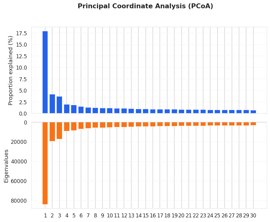 The scree plot displays the amount of variability in the data that is explained by each PCoA axis. This allows you to understand how well the two-dimensional plot represents the overall differences in community composition across all the samples. Axes that explain more of the variability are more important for understanding the main factors that cause the samples to be different from each other.
**Why it's useful**
* **Judge how well the 2D plot summarizes the data:** if PCoA1 and PCoA2 explain a large share of variation, the ordination is a strong summary; if they explain only a small share, the plot still helps but represents only part of the full differences.
* **See whether differences come from one strong pattern or many:** if PCoA1 explains far more than the others, one dominant source separates the samples; if variation is spread across many axes, the differences are more complex and distributed, rather than driven by a single gradient.
The scree plot displays the amount of variability in the data that is explained by each PCoA axis. This allows you to understand how well the two-dimensional plot represents the overall differences in community composition across all the samples. Axes that explain more of the variability are more important for understanding the main factors that cause the samples to be different from each other.
**Why it's useful**
* **Judge how well the 2D plot summarizes the data:** if PCoA1 and PCoA2 explain a large share of variation, the ordination is a strong summary; if they explain only a small share, the plot still helps but represents only part of the full differences.
* **See whether differences come from one strong pattern or many:** if PCoA1 explains far more than the others, one dominant source separates the samples; if variation is spread across many axes, the differences are more complex and distributed, rather than driven by a single gradient.
## Ordination and statistical test tables
Scroll past the of the output page to download intermediate files and statistical summaries of the Beta-diversity Analysis module
| Table | What it contains |
| :--------------------------------------------- | :--------------------------------------------------------------------------------------------------------------------------------------------- |
| **PCoA: proportion explained and eigenvalues** | The numerical form of the scree plot: the proportion of variation explained by each PCoA axis and its eigenvalue. |
| **PCoA: sample coordinates** | The PCoA coordinates of every sample across 150 axes. The first two columns are the coordinates used to place the dots on the ordination plot. |
| **PERMANOVA summary** | Sample size, number of groups, pseudo-F statistic, p-value, and permutation count for the overall test. |
| **ANOSIM summary** | Sample size, number of groups, R statistic, p-value, and permutation count for the overall test. |
| **Pairwise PERMANOVA / ANOSIM results** | Each pairwise group comparison: group names, sample sizes, test statistics, p-values, FDR-adjusted q-values, and permutation counts. |
## Recommended parameters
| Parameter | Recommended value |
| :------------------------------------------------------------- | :----------------------------------------------------------------------------------------------------------------------------------------------------------------------------------------------------------------------------------------------------------------------------------------------------------------------------------------------------------------------------------------------------------------------------------------------------------------------------------------------------------------------------------- |
| Analysis Metric | `relative_abundance` |
| Taxonomic Rank | `species` |
| Data Table Pre-processing Method | - `raw` if samples have comparable read depths
- `filter` if a few samples have notably lower read depth than the rest of the cohort
- `rarefaction` to standardize the whole cohort to a common read depth
Sequencing depth heavily affects output with presence-absence Beta-diversity metric (e.g:`Jaccard`).
Compositional-aware distances (e.g: `Braycurtis`or `Aitchison` ) are robust to variability in sequencing depth. |
| Read Depth | - When using `rarefaction`, use the [Rarefaction module](/DAP_docs/rarefaction-on-the-dap) to detect an optimal read depth to avoid discarding too many samples. Samples below it are discarded, so depth trades against sample size.
- With `filter`, set a threshold that removes only the samples with notably lower depth. The retention plot helps spot them.
|
| Feature Relative Abundance Threshold | `0.0001` |
| Feature Prevalence Threshold | - `0` with `Jaccard`
- `0.01` to `0.05` with `Bray Curtis`
- `0.05` to `0.1 ` with `Aitchison`
Use minimal but nonzero filtering for Jaccard, since each detected taxon contributes equally regardless of abundance and rare detections can be noise-sensitive. Apply modest filtering for Bray–Curtis and stronger filtering before conventional Aitchison analysis, where high sparsity makes results sensitive to zero replacement rather than measured relative abundances. |
| Beta Diversity Metric | - `Aitchison` or `Bray-Curtis` : you care about differences in *relative community structure*
- `Jaccard : `your question is whether samples differ in *which taxa are detected*
|
| Centroid Method (if available) | `median`
|
| Number of Components | - `2` when the first two axes capture most of the variation
- `3` if the third PCoA axis explains nearly as much as the second (use the PCoA scree plot).
Note: A static 3D plot gets easily crowded with many samples.
|
| Grouping Variable | Categorical metadata of interest.
Grouping defines the groups compared by PERMANOVA and ANOSIM. Avoid variables with very few samples per category. |
| Drop samples with missing metadata values in grouping variable | ✅ |
| Number of Permutations | - Exploring: `999`
- For more confidence in the p-value, especially near your threshold: `9999`
With `999` permutations the smallest p-value obtainable is `0.001`. |
| Max Ellipses | Number of groups in your grouping variable (up to about `5`) |
| Shape Variable | Optional second categorical variable. For example, color by `treatment` and shape by `timepoint` to see whether groups separate only at later timepoints. |
| Confidence Level | - `0.95` as standard.
- `0.70` for tighter ellipses on crowded plots.
|
| Parameter | Recommended value |
| :------------------------------------------------------------- | :----------------------------------------------------------------------------------------------------------------------------------------------------------------------------------------------------------------------------------------------------------------------------------------------------------------------------------------------------------------------------------------------------------------------------------------------------------------------------------------------------------------------------------- |
| Analysis Metric | `relative_abundance` |
| Taxonomic Rank | `species` |
| Data Table Pre-processing Method | - `raw` if samples have comparable read depths
- `filter` if a few samples have notably lower read depth than the rest of the cohort
- `rarefaction` to standardize the whole cohort to a common read depth
Sequencing depth heavily affects output with presence-absence Beta-diversity metric (e.g:`Jaccard`).
Compositional-aware distances (e.g: `Braycurtis`or `Aitchison` ) are robust to variability in sequencing depth. |
| Read Depth | - When using `rarefaction`, use the [Rarefaction module](/DAP_docs/rarefaction-on-the-dap) to detect an optimal read depth to avoid discarding too many samples. Samples below it are discarded, so depth trades against sample size.
- With `filter`, set a threshold that removes only the samples with notably lower depth. The retention plot helps spot them.
|
| Feature Relative Abundance Threshold | `0.0001` |
| Feature Prevalence Threshold | - `0` with `Jaccard`
- `0.01` to `0.05` with `Bray Curtis`
- `0.05` to `0.1 ` with `Aitchison`
Use minimal but nonzero filtering for Jaccard, since each detected taxon contributes equally regardless of abundance and rare detections can be noise-sensitive. Apply modest filtering for Bray–Curtis and stronger filtering before conventional Aitchison analysis, where high sparsity makes results sensitive to zero replacement rather than measured relative abundances. |
| Beta Diversity Metric | - `Aitchison` or `Bray-Curtis` : you care about differences in *relative community structure*
- `Jaccard : `your question is whether samples differ in *which taxa are detected*
|
| Centroid Method (if available) | `median` |
| Number of Components | - `2` when the first two axes capture most of the variation
- `3` if the third PCoA axis explains nearly as much as the second (use the PCoA scree plot).
Note: A static 3D plot gets easily crowded with many samples.
|
| Grouping Variable | Categorical metadata of interest.
Grouping defines the groups compared by PERMANOVA and ANOSIM. Avoid variables with very few samples per category. |
| Drop samples with missing metadata values in grouping variable | ✅ |
| Number of Permutations | - Exploring: `999`
- For more confidence in the p-value, especially near your threshold: `9999`
With `999` permutations the smallest p-value obtainable is `0.001`. |
| Max Ellipses | Number of groups in your grouping variable (up to about `5`) |
| Shape Variable | Optional second categorical variable. For example, color by `treatment` and shape by `timepoint` to see whether groups separate only at later timepoints. |
| Confidence Level | - `0.95` as standard.
- `0.70` for tighter ellipses on crowded plots.
|
| Parameter | Recommended value |
| :------------------------------------------------------------- | :----------------------------------------------------------------------------------------------------------------------------------------------------------------------------------------------------------------------------------------------------------------------------------------------------------------------------------------------------------------------------------------------------------------------------------------------------------------------------------------------------------------------------------- |
| Analysis Metric | `relative_abundance` |
| Taxonomic Rank | `genus` |
| Data Table Pre-processing Method | - `raw` if samples have comparable read depths
- `filter` if a few samples have notably lower read depth than the rest of the cohort
- `rarefaction` to standardize the whole cohort to a common read depth
Sequencing depth heavily affects output with presence-absence Beta-diversity metric (e.g:`Jaccard`).
Compositional-aware distances (e.g: `Braycurtis`or `Aitchison` ) are robust to variability in sequencing depth. |
| Read Depth | - When using `rarefaction`, use the [Rarefaction module](/DAP_docs/rarefaction-on-the-dap) to detect an optimal read depth to avoid discarding too many samples. Samples below it are discarded, so depth trades against sample size.
- With `filter`, set a threshold that removes only the samples with notably lower depth. The retention plot helps spot them.
|
| Feature Relative Abundance Threshold | `0.0001` |
| Feature Prevalence Threshold | - `0` with `Jaccard`
- `0.01` to `0.05` with `Bray Curtis`
- `0.05` to `0.1 ` with `Aitchison`
Use minimal but nonzero filtering for Jaccard, since each detected taxon contributes equally regardless of abundance and rare detections can be noise-sensitive. Apply modest filtering for Bray–Curtis and stronger filtering before conventional Aitchison analysis, where high sparsity makes results sensitive to zero replacement rather than measured relative abundances. |
| Beta Diversity Metric | - `Aitchison` or `Bray-Curtis` : you care about differences in *relative community structure*
- `Jaccard : `your question is whether samples differ in *which taxa are detected*
|
| Centroid Method (if available) | `median` |
| Number of Components | - `2` when the first two axes capture most of the variation
- `3` if the third PCoA axis explains nearly as much as the second (use the PCoA scree plot).
Note: A static 3D plot gets easily crowded with many samples.
|
| Grouping Variable | Categorical metadata of interest.
Grouping defines the groups compared by PERMANOVA and ANOSIM. Avoid variables with very few samples per category. |
| Drop samples with missing metadata values in grouping variable | ✅ |
| Number of Permutations | - Exploring: `999`
- For more confidence in the p-value, especially near your threshold: `9999`
With `999` permutations the smallest p-value obtainable is `0.001`. |
| Max Ellipses | Number of groups in your grouping variable (up to about `5`) |
| Shape Variable | Optional second categorical variable. For example, color by `treatment` and shape by `timepoint` to see whether groups separate only at later timepoints. |
| Confidence Level | - `0.95` as standard.
- `0.70` for tighter ellipses on crowded plots.
|
| Parameter | Recommended value |
| :------------------------------------------------------------- | :----------------------------------------------------------------------------------------------------------------------------------------------------------------------------------------------------------------------------------------------------------------------------------------------------------------------------------------------------------------------------------------------------------------------------------------------------------------------------------------------------------------------------------- |
| Analysis Metric | `relative_abundance` |
| Taxonomic Rank | `species` |
| Data Table Pre-processing Method | - `raw` if samples have comparable read depths
- `filter` if a few samples have notably lower read depth than the rest of the cohort
- `rarefaction` to standardize the whole cohort to a common read depth.
Sequencing depth heavily affects output with presence-absence Beta-diversity metric (e.g:`Jaccard`).
Compositional-aware distances (e.g: `Braycurtis`or `Aitchison` ) are robust to variability in sequencing depth. |
| Read Depth | - When using `rarefaction`, use the [Rarefaction module](/DAP_docs/rarefaction-on-the-dap) to detect an optimal read depth to avoid discarding too many samples. Samples below it are discarded, so depth trades against sample size.
- With `filter`, set a threshold that removes only the samples with notably lower depth. The retention plot helps spot them.
|
| Feature Relative Abundance Threshold | `0.0001` |
| Feature Prevalence Threshold | - `0` with `Jaccard`
- `0.01` to `0.05` with `Bray Curtis`
- `0.05` to `0.1 ` with `Aitchison`
Use minimal but nonzero filtering for Jaccard, since each detected taxon contributes equally regardless of abundance and rare detections can be noise-sensitive. Apply modest filtering for Bray–Curtis and stronger filtering before conventional Aitchison analysis, where high sparsity makes results sensitive to zero replacement rather than measured relative abundances. |
| Beta Diversity Metric | - `Aitchison` or `Bray-Curtis` : you care about differences in *relative community structure*
- `Jaccard : `your question is whether samples differ in *which taxa are detected*
|
| Centroid Method (if available) | `median` |
| Number of Components | - `2` when the first two axes capture most of the variation
- `3` if the third PCoA axis explains nearly as much as the second (use the PCoA scree plot).
Note: A static 3D plot gets easily crowded with many samples.
|
| Grouping Variable | Categorical metadata of interest.
Grouping defines the groups compared by PERMANOVA and ANOSIM. Avoid variables with very few samples per category. |
| Drop samples with missing metadata values in grouping variable | ✅ |
| Number of Permutations | - Exploring: `999`
- For more confidence in the p-value, especially near your threshold: `9999`
With `999` permutations the smallest p-value obtainable is `0.001`. |
| Max Ellipses | Number of groups in your grouping variable (up to about `5`) |
| Shape Variable | Optional second categorical variable. For example, color by `treatment` and shape by `timepoint` to see whether groups separate only at later timepoints. |
| Confidence Level | - `0.95` as standard.
- `0.70` for tighter ellipses on crowded plots.
|
| Parameter | Recommended value |
| :------------------------------------------------------------- | :------------------------------------------------------------------------------------------------------------------------------------------------------------------------------------------------------------------------------------------------------- |
| Analysis Metric | `relative_abundance` |
| Data Table Pre-processing Method | `raw` |
| Read Depth | - With `filter`, set a threshold that removes only the samples with notably lower depth. The retention plot helps spot them.
|
| Feature Relative Abundance Threshold | `0.0001` |
| Feature Prevalence Threshold | - `0` with `Jaccard`
- `0.01` to `0.05` with `Bray Curtis`
- `0.05` to `0.1 ` with `Aitchison`
|
| Beta Diversity Metric | - `Aitchison` or `Bray-Curtis` : you care about differences in *relative functional composition*
- `Jaccard : `your question is whether samples differ in *which functions are detected*
|
| Number of Components | - `2` when the first two axes capture most of the variation
- `3` if the third PCoA axis explains nearly as much as the second (use the PCoA scree plot).
Note: A static 3D plot gets easily crowded with many samples.
|
| Grouping Variable | Categorical metadata of interest.
Grouping defines the groups compared by PERMANOVA and ANOSIM. Avoid variables with very few samples per category. |
| Drop samples with missing metadata values in grouping variable | ✅ |
| Number of Permutations | - Exploring: `999`
- For more confidence in the p-value, especially near your threshold: `9999`
With `999` permutations the smallest p-value obtainable is `0.001`. |
| Max Ellipses | Number of groups in your grouping variable (up to about `5`) |
| Shape Variable | Optional second categorical variable. For example, color by `treatment` and shape by `timepoint` to see whether groups separate only at later timepoints. |
| Confidence Level | - `0.95` as standard.
- `0.70` for tighter ellipses on crowded plots.
|
| Parameter | Recommended value |
| :------------------------------------------------------------- | :----------------------------------------------------------------------------------------------------------------------------------------------------------------------------------------------------------------------------------------------------------------------------------------------------------------------------------------------------------------------------------------- |
| Analysis Metric | `cellular_abundance` |
| Data Table Pre-processing Method | `raw` |
| Read Depth | - When using `rarefaction`, use the [Rarefaction module](/DAP_docs/rarefaction-on-the-dap) to detect an optimal read depth to avoid discarding too many samples. Samples below it are discarded, so depth trades against sample size.
- With `filter`, set a threshold that removes only the samples with notably lower depth. The retention plot helps spot them.
|
| Feature Relative Abundance Threshold | `0.0001` |
| Feature Prevalence Threshold | - `0` with `Jaccard`
- `0.01` to `0.05` with `Bray Curtis`
- `0.05` to `0.1 ` with `Aitchison`
|
| Beta Diversity Metric | - `Bray-Curtis` or `Aitchison`: you care about differences in *relative functional module composition*
- `Jaccard : `your question is whether samples differ in *which functional modules or pathways are detected*
|
| Number of Components | - `2` when the first two axes capture most of the variation
- `3` if the third PCoA axis explains nearly as much as the second (use the PCoA scree plot).
Note: A static 3D plot gets easily crowded with many samples.
|
| Grouping Variable | Categorical metadata of interest.
Grouping defines the groups compared by PERMANOVA and ANOSIM. Avoid variables with very few samples per category. |
| Drop samples with missing metadata values in grouping variable | ✅ |
| Number of Permutations | - Exploring: `999`
- For more confidence in the p-value, especially near your threshold: `9999`
With `999` permutations the smallest p-value obtainable is `0.001`. |
| Max Ellipses | Number of groups in your grouping variable (up to about `5`) |
| Shape Variable | Optional second categorical variable. For example, color by `treatment` and shape by `timepoint` to see whether groups separate only at later timepoints. |
| Confidence Level | - `0.95` as standard.
- `0.70` for tighter ellipses on crowded plots.
|
| Parameter | Recommended value |
| :------------------------------------------------------------- | :----------------------------------------------------------------------------------------------------------------------------------------------------------------------------------------------------------------------------------------------------------------------------------------------------------------------------------------------------------------------------------------- |
| Analysis Metric | `relative_abundance` |
| Data Table Pre-processing Method | `raw` |
| Read Depth | - When using `rarefaction`, use the [Rarefaction module](/DAP_docs/rarefaction-on-the-dap) to detect an optimal read depth to avoid discarding too many samples. Samples below it are discarded, so depth trades against sample size.
- With `filter`, set a threshold that removes only the samples with notably lower depth. The retention plot helps spot them.
|
| Feature Relative Abundance Threshold | `0.0001` |
| Feature Prevalence Threshold | - `0` with `Jaccard`
- `0.01` to `0.05` with `Bray Curtis`
- `0.05` to `0.1 ` with `Aitchison`
|
| Beta Diversity Metric | - `Aitchison` or `Bray-Curtis` : you care about differences in *relative resistance/virulence gene composition*
- `Jaccard : `your question is whether samples differ in *which resistance or virulence genes are detected*
|
| Number of Components | - `2` when the first two axes capture most of the variation
- `3` if the third PCoA axis explains nearly as much as the second (use the PCoA scree plot).
Note: A static 3D plot gets easily crowded with many samples.
|
| Grouping Variable | Categorical metadata of interest.
Grouping defines the groups compared by PERMANOVA and ANOSIM. Avoid variables with very few samples per category. |
| Drop samples with missing metadata values in grouping variable | ✅ |
| Number of Permutations | - Exploring: `999`
- For more confidence in the p-value, especially near your threshold: `9999`
With `999` permutations the smallest p-value obtainable is `0.001`. |
| Max Ellipses | Number of groups in your grouping variable (up to about `5`) |
| Shape Variable | Optional second categorical variable. For example, color by `treatment` and shape by `timepoint` to see whether groups separate only at later timepoints. |
| Confidence Level | - `0.95` as standard.
- `0.70` for tighter ellipses on crowded plots.
|
## Parameter reference
The categorical metadata column that defines the groups you want to compare. It plays two roles at once: it sets the **color** of the points in the ordination plot (one color per category), and it defines the groups that the **PERMANOVA / ANOSIM** tests use to ask whether community composition actually differs between them. Choose the variable that encodes your biological question, the factor you expect to separate the microbial communities (for example, case versus control, or body site).
* **Options** · Categorical variables from the metadata table associated with the query used to create the analysis
* **Default** · `None`: no grouping is applied, all samples share one color and the plot shows their overall spread without group comparisons. Choose a grouping variable to color samples by metadata and compare groups.
* **Suggested** · A categorical variable relevant to your study design, such as `treatment`, `disease status`, `condition`, `body site`, `cohort`, or `time point`. Avoid variables with too many categories or categories represented by very few samples, these clutter the plot and reduce the reliability of statistical testing.
The rule used to turn any two microbial profiles into a single **distance**, a number summarizing how different two samples are. Computing it for every pair of samples produces the **distance matrix** that everything downstream is built on: the ordination plot and the PERMANOVA / ANOSIM tests. The choice matters because each metric weighs the data differently: some respond to differences in **abundance**, some only to which features are **present or absent**, and some are designed for **compositional** data (where sequencing measures relative, not absolute, abundances).
* **Options** · 23 metrics
* **Default** · `Euclidean`
* **Suggested** · Match the metric to your question and feature type:
| Goal | Feature type | Metric | Why | Note |
| :------------------------------------------------ | :--------------------------------- | :---------------------------- | :---------------------------------------------------------------------- | :------------------------------------------------------------------- |
| Differ in overall composition based on abundance? | Relative abundance | **Bray-Curtis** | Popular, intuitive abundance-based distance; a safe default | Sensitive to abundance differences; doesn't address compositionality |
| Contain different taxa, regardless of abundance? | Presence/absence | **Jaccard** or **Dice** | Focuses on shared versus non-shared features | Ignores abundance, so rare and abundant taxa count equally |
| Differ as compositional profiles? | Relative abundance / compositional | **Aitchison** | Built for compositional data; compares log-ratios between features | Needs appropriate zero handling before the log-ratio transformation |
| Are low-abundance features important? | Counts or relative abundance | **Canberra** | Gives more weight to proportional differences in low-abundance features | Sensitive to zeros, noise, and very rare features |
| Have similar functional profile shapes? | Functional profiles | **Cosine** or **Correlation** | Compares overall profile shape rather than direct abundance | More exploratory; depends heavily on preprocessing and scaling |
*Available only when the Beta-diversity Metric is* `Aitchison`
* The Aitchison metric first applies a **CLR (centered log-ratio) transformation**: within each sample, every feature's abundance is divided by a single per-sample reference value and then log-transformed, which removes the compositional constraint and makes samples comparable. This parameter chooses which summary statistic is used as that reference value, so it controls how each sample is centered before distances are computed.
* **Options** · `mean`, `median`
* **Default** · `mean`
* **Suggested**
* `mean`: the geometric mean of abundances (the standard CLR choice). Best when the data is fairly clean and most taxa carry meaningful signal.
* `median`: more robust to outliers and noisy low-abundance taxa, often useful for sparse microbiome data.
The number of ordination axes shown in the plot. An ordination method compresses the full distance matrix into a handful of axes, ordered by how much sample-to-sample variation each one captures; this sets how many of those leading axes are displayed.
* **Options** · `2` (2D) or `3` (3D)
* **Default** · `2`
* **Suggested**:
* `2`: a standard 2D scatter plot: easier to read, annotate, and export, and usually enough when the first two components capture most variation.
* `3`: when the first two components don't capture enough structure, or an extra axis reveals separation hidden in 2D. Shown as a static 3D plot.
Controls what happens to samples that have **no value** for the grouping variable (missing metadata).
* **Default** · `TRUE` (samples with missing values are dropped)
* **Enabled**: samples with missing metadata are removed before the analysis runs. The distance matrix, ordination, and tests are computed only on samples with a valid group, keeping comparisons clean.
* **Disabled**: samples with missing values are kept and assigned to a separate `NaN_group`, appearing as their own group and included in calculations. **Suggested** · **Enable** to compare well-defined groups, run PERMANOVA, or produce a clean publication plot (missing values can otherwise distort group centroids, within-group spread, and test results). **Disable** when it's useful to see where unlabelled samples fall in the ordination, for example to check whether they cluster with any known group.
*Note:* *ellipses are drawn only when Number of Components is set to '2'* The maximum number of group **confidence ellipses** drawn on the 2D plot. Each ellipse summarizes one group's center and spread in the ordination space, making it easy to see at a glance whether groups overlap or pull apart. Ellipses are drawn only for groups present in the plotted data with an assigned color; if more groups are eligible than this maximum, only the first ones in plotting order get an ellipse. **Options** · `0` to `10` **Default** · `0` **Suggested** · With few, well-separated groups (≤5), showing all is fine. For more complex datasets, limiting the number improves readability.
How much of each group its ellipse covers: the percentage of that group's samples expected to fall inside it. Higher values draw wider ellipses; lower values draw tighter ones. **Options** · `50` to `99%` **Default** · `95%`
This parameter only affects the **visualization** of group ellipses. It does not change the beta-diversity calculation, sample positions, or statistical results. Ellipses are visual aids: don't read them as strict statistical boundaries or as proof of group separation.
The number of random permutations used to calculate significance for **PERMANOVA** or **ANOSIM**. The group labels are shuffled this many times (with the distances held fixed) to build a **null distribution**, the range of group separation you'd expect to see if the labels were random. The separation actually observed is then compared against it to produce the p-value. **Options** · `99` to `10000` **Default** · `999` **Suggested** · Use `999` for standard exploratory analysis. Use `4999` or `9999` when results will be reported formally, or when the p-value is close to the significance threshold. Higher values give more precise p-values but take longer.
This parameter affects only the significance testing, it does not change the distances, the ordination, or sample positions.
An optional categorical metadata column mapped to different point **shapes**, letting you overlay a second factor on top of the color-coded grouping variable. It's purely visual, it doesn't change the distance matrix, the ordination, or the statistics. **Options** · Metadata variables from the metadata table associated with the query used to create the analysis **Default** · `None` (all samples share the same shape) **Suggested** · A categorical variable that adds context, such as `sex`, `cohort`, `sample type`, `time point`, or `body site`. For example, with samples colored by `treatment`, the shape could show which cohort or collection site each came from.
## References
* Anderson, M. (2001). "A new method for non-parametric multivariate analysis of variance." Austral Ecology, 26(1), 32-46. [https://dx.doi.org/10.1111/j.1442-9993.2001.01070.pp.x](https://dx.doi.org/10.1111/j.1442-9993.2001.01070.pp.x)
* Anderson, M. (2014). "Permutational Multivariate Analysis of Variance (PERMANOVA)." Wiley StatsRef: Statistics Reference Online. [https://doi.org/10.1002/9781118445112.stat07841](https://doi.org/10.1002/9781118445112.stat07841)
* **Jaccard Index.** Jaccard, P. (1901). "Étude comparative de la distribution florale dans une portion des Alpes et des Jura." Bulletin de la Société vaudoise des sciences naturelles, 37(142), 547-579. Jaccard, P. (1912). "The Distribution of the Flora in the Alpine Zone. 1." New Phytologist, 11(2), 37-50. doi:10.1111/j.1469-8137.1912.tb05611.x
* **Bray-Curtis Dissimilarity.** Bray, J. R. & Curtis, J. T. (1957). "An ordination of the upland forest communities of southern Wisconsin." Ecological Monographs, 27, 325-349.