> ## Documentation Index
> Fetch the complete documentation index at: https://docs.cosmosid.com/llms.txt
> Use this file to discover all available pages before exploring further.

# Overview

> What Principal Component Analysis does, how it condenses many features into a few axes, and why it's useful for microbiome data.

## What is Principal Component Analysis?

Principal Component Analysis (PCA) reduces the many microbial features per sample down to a few principal components (PCs), projecting the data onto fewer dimensions so that the main trends and patterns among samples become visible on a 2D or 3D plot. It finds this structure without any prior knowledge of the groups or variables associated with the samples.

## How does it work?

<Frame caption="Here I would put an image similar to what I already have for Overviews of alpha- and beta-diversity">
  <img src="https://mintcdn.com/cmbio/9IPlECfVJPWdo6z4/DAP_docs/DAP-images/pca_biplot_example.png?fit=max&auto=format&n=9IPlECfVJPWdo6z4&q=85&s=2b5db348c17b395b608535a56faca573" alt="Pca Biplot Example" width="1329" height="1048" data-path="DAP_docs/DAP-images/pca_biplot_example.png" />
</Frame>

<Steps>
  <Step title="Start from the Data Table">
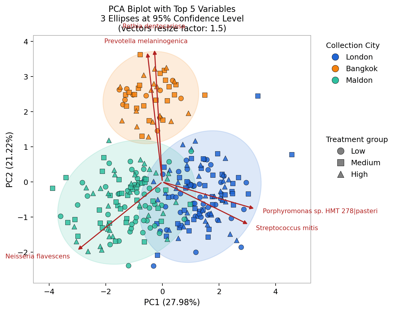    Each sample is a vector describing the abundances of many features  often hundreds or thousands of taxa. Comparing samples across that many dimensions directly is impractical, since only two or three axes can be visualized at once.
  </Step>

  <Step title="Find the strongest pattern of variation (PC1)">
    Features rarely vary independently — subsets of taxa tend to co-vary across samples. PCA finds the single combination of features along which samples are most spread out. This becomes the first principal component (**PC1**): the axis reflecting the largest source of variation.
  </Step>

  <Step title="Find the next patterns">
    PCA then finds the next strongest pattern, independent of the first, giving **PC2**, and so on. Each further component captures a smaller, distinct portion of the remaining variation.
  </Step>

  <Step title="Reposition the samples">
    Each sample receives a coordinate along these new axes (its *score*), which places it in the plot. How much each original feature contributes to an axis is its *loading* — the loadings reveal which taxa define each component.
  </Step>
</Steps>

## Why is it useful?

PCA condenses hundreds or thousands of features of a microbial profile into a few interpretable axes. For example, it can:

* **Reveal sample structure** — show whether samples separate into groups based on overall composition, without testing any feature individually.
* **Identify the features behind that structure** — through the loadings, point to which features contribute most to the separation seen in the plot.
* **Summarize variation compactly** — express the dominant patterns with a few components, each accounting for a known proportion of the total variation.