> ## Documentation Index
> Fetch the complete documentation index at: https://docs.cosmosid.com/llms.txt
> Use this file to discover all available pages before exploring further.
# Pre-processing Parameters
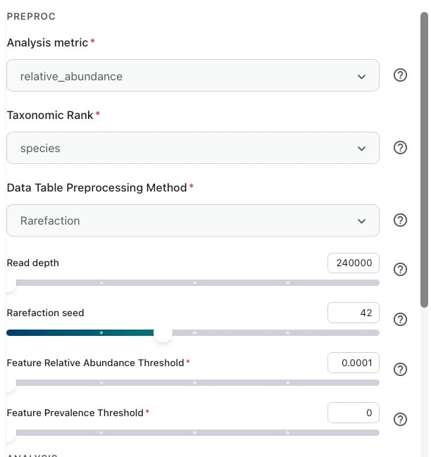
Each Analysis Module's Parameter panel has a **PREPROC** section for pre-processing parameters. These parameters control how the feature table is transformed, filtered, or aggregated, across both samples and features, before it is used as the module's input.
 ## Analysis Metric
Controls the metric by which a feature abundances are represented and normalized in the Data Table that will be processed by the Analysis Modules. The Analysis Metricsavailable in the Cosmos-Hub 2.0 depend on the type of profiles (taxonomic or functional) that were used to build the cohort for the current Analysis Project.
### Analyses metrics in the Cosmos-Hub 2.0:
**Analysis Metrics Available for all Cosmos-Hub Taxonomic Profilers and for Host-agnostic Functional Profiling**
* `counts`: the number of sequencing reads assigned to each taxon or functional gene in each sample.
* `relative_abundance`: the fraction of each sample's microbial profile represented by that taxon or function.
In most microbiome analyses, `relative_abundance` is the more intuitive choice because it describes community composition: for example, whether a taxon makes up 1%, 10%, or 50% of a sample. It also makes samples easier to compare when they were sequenced at different depths, because each sample is rescaled to the same total.
**Low-depth samples and relative abundance.** Relative abundance is calculated by normalizing each feature's read count against the total number of reads in that sample. When a sample has a much lower read depth than the rest of the cohort, its relative abundance estimates can be unstable—small fluctuations in a handful of reads can cause large swings in the reported proportions. This makes comparisons across samples misleading, as a taxon appearing at 10% in a low-depth sample (e.g. 50 out of 500 reads) carries far less confidence than the same 10% in a high-depth sample (e.g. 5,000 out of 50,000 reads). Before comparing relative abundance distributions, check for outlier samples with disproportionately low read depth and consider whether they should be filtered out or flagged.
Use `counts` only when the analysis method expects read counts or when the number of reads assigned to a feature is itself important. Keep in mind that read counts are affected by sequencing depth: a sample with more total reads may have higher counts simply because it was sequenced more deeply, not necessarily because the organism is more abundant in the original biological sample.
**Analysis Metrics available for Champ Functional Profiling (KEGG KO and Modules, GBM, GMM):**
* `cellular_abundance`: represents the relative percentage of species that are able to perform a given function in the microbiome community
## Taxonomic Rank
This pre-processing parameter performs a *Feature aggregation operation* on the input Data Table
Sets the taxonomic level at which features (rows) in the Data Table are aggregated, for example species, genus, family, or phylum. This parameter applies only to taxonomic profiles. Choosing a higher Taxonomic Rank collapses all features that share the same classification at that level into a single row, summing their abundance values.
Collapsing the same Taxonomic Data Table expressed in counts by Genus
| Feature | Sample A | Sample B | Sample C |
| ------------------------- | -------- | -------- | -------- |
| *Lactobacillus crispatus* | 150 | 200 | 90 |
| *Lactobacillus iners* | 80 | 50 | 110 |
| *Gardnerella vaginalis* | 50 | 120 | 60 |
| *Gardnerella leopoldii* | 20 | 30 | 10 |
| *Prevotella bivia* | 40 | 10 | 70 |
| Feature | Sample A | Sample B | Sample C |
| --------------- | -------- | -------- | -------- |
| *Lactobacillus* | 230 | 250 | 200 |
| *Gardnerella* | 70 | 150 | 70 |
| *Prevotella* | 40 | 10 | 70 |
## Data Table Pre-processing Method
This pre-processing parameter acts on *Sample filter and Feature filtering* on the input Data Table
**Data Table Pre-processing: Method** controls pre-processing at the sample-depth level. It determines whether low-depth samples are filtered and whether retained samples are rarefied to a common read depth. This helps make samples more comparable when sequencing depth differs, particularly for analyses based on feature detection, such as observed richness.
Three strategies are available in the Cosmos-Hub 2.0:
* `Raw`: applies no sample pre-processing. All samples in the Data Table are kept, regardless sample sequencing depth.
* `Filter`: removes samples with a sequencing depth falling below the chosen **Read depth** threshold. Selecting this method reveals the **Read depth** parameter for setting the lower sequencing-depth threshold.
This Data Table Pre-processing Method operates a *Sample filter* operation on the Data Table
* `Rarefaction`: randomly subsamples reads from each sample down to the selected Read Depth, so that all samples in the table share the same sequencing depth.
This method applies a **Sample filter** and a **Data transformation** to the Data Table.
Rarefaction and Filtering strategies are currently available for profiles for which Analysis Metric `counts`is available.
**Filtering or Rarefaction?**
* Filter out samples when depth is a clear outlier vs. the rest of the batch, falls below what's needed to detect your taxa of interest, or shows a r[arefaction curve](DAP_docs/rarefaction-on-the-dap) that hasn't plateaued.
* Rarefaction discards reads from remaining samples to equalize depth, which can zero out sparse taxa/genes. Use rarefaction when the Analysis module you are running is depth-sensitive (e.g: Alpha diversity with observed richness or Beta Diversity with a presence-absence distance metric like Jaccard.
#### **Rarefaction Seed** *(available when Data Table Pre-processing Method is set to Rarefaction)*
Data table rarefaction works by *randomly* subsampling reads from each sample down to a common depth. Because the selection is random, running the same analysis twice could pick a slightly different set of reads each time, which means your results (diversity values, which rare features survive, and so on) could slightly vary from run to run on identical data.
## Analysis Metric
Controls the metric by which a feature abundances are represented and normalized in the Data Table that will be processed by the Analysis Modules. The Analysis Metricsavailable in the Cosmos-Hub 2.0 depend on the type of profiles (taxonomic or functional) that were used to build the cohort for the current Analysis Project.
### Analyses metrics in the Cosmos-Hub 2.0:
**Analysis Metrics Available for all Cosmos-Hub Taxonomic Profilers and for Host-agnostic Functional Profiling**
* `counts`: the number of sequencing reads assigned to each taxon or functional gene in each sample.
* `relative_abundance`: the fraction of each sample's microbial profile represented by that taxon or function.
In most microbiome analyses, `relative_abundance` is the more intuitive choice because it describes community composition: for example, whether a taxon makes up 1%, 10%, or 50% of a sample. It also makes samples easier to compare when they were sequenced at different depths, because each sample is rescaled to the same total.
**Low-depth samples and relative abundance.** Relative abundance is calculated by normalizing each feature's read count against the total number of reads in that sample. When a sample has a much lower read depth than the rest of the cohort, its relative abundance estimates can be unstable—small fluctuations in a handful of reads can cause large swings in the reported proportions. This makes comparisons across samples misleading, as a taxon appearing at 10% in a low-depth sample (e.g. 50 out of 500 reads) carries far less confidence than the same 10% in a high-depth sample (e.g. 5,000 out of 50,000 reads). Before comparing relative abundance distributions, check for outlier samples with disproportionately low read depth and consider whether they should be filtered out or flagged.
Use `counts` only when the analysis method expects read counts or when the number of reads assigned to a feature is itself important. Keep in mind that read counts are affected by sequencing depth: a sample with more total reads may have higher counts simply because it was sequenced more deeply, not necessarily because the organism is more abundant in the original biological sample.
**Analysis Metrics available for Champ Functional Profiling (KEGG KO and Modules, GBM, GMM):**
* `cellular_abundance`: represents the relative percentage of species that are able to perform a given function in the microbiome community
## Taxonomic Rank
This pre-processing parameter performs a *Feature aggregation operation* on the input Data Table
Sets the taxonomic level at which features (rows) in the Data Table are aggregated, for example species, genus, family, or phylum. This parameter applies only to taxonomic profiles. Choosing a higher Taxonomic Rank collapses all features that share the same classification at that level into a single row, summing their abundance values.
Collapsing the same Taxonomic Data Table expressed in counts by Genus
| Feature | Sample A | Sample B | Sample C |
| ------------------------- | -------- | -------- | -------- |
| *Lactobacillus crispatus* | 150 | 200 | 90 |
| *Lactobacillus iners* | 80 | 50 | 110 |
| *Gardnerella vaginalis* | 50 | 120 | 60 |
| *Gardnerella leopoldii* | 20 | 30 | 10 |
| *Prevotella bivia* | 40 | 10 | 70 |
| Feature | Sample A | Sample B | Sample C |
| --------------- | -------- | -------- | -------- |
| *Lactobacillus* | 230 | 250 | 200 |
| *Gardnerella* | 70 | 150 | 70 |
| *Prevotella* | 40 | 10 | 70 |
## Data Table Pre-processing Method
This pre-processing parameter acts on *Sample filter and Feature filtering* on the input Data Table
**Data Table Pre-processing: Method** controls pre-processing at the sample-depth level. It determines whether low-depth samples are filtered and whether retained samples are rarefied to a common read depth. This helps make samples more comparable when sequencing depth differs, particularly for analyses based on feature detection, such as observed richness.
Three strategies are available in the Cosmos-Hub 2.0:
* `Raw`: applies no sample pre-processing. All samples in the Data Table are kept, regardless sample sequencing depth.
* `Filter`: removes samples with a sequencing depth falling below the chosen **Read depth** threshold. Selecting this method reveals the **Read depth** parameter for setting the lower sequencing-depth threshold.
This Data Table Pre-processing Method operates a *Sample filter* operation on the Data Table
* `Rarefaction`: randomly subsamples reads from each sample down to the selected Read Depth, so that all samples in the table share the same sequencing depth.
This method applies a **Sample filter** and a **Data transformation** to the Data Table.
Rarefaction and Filtering strategies are currently available for profiles for which Analysis Metric `counts`is available.
**Filtering or Rarefaction?**
* Filter out samples when depth is a clear outlier vs. the rest of the batch, falls below what's needed to detect your taxa of interest, or shows a r[arefaction curve](DAP_docs/rarefaction-on-the-dap) that hasn't plateaued.
* Rarefaction discards reads from remaining samples to equalize depth, which can zero out sparse taxa/genes. Use rarefaction when the Analysis module you are running is depth-sensitive (e.g: Alpha diversity with observed richness or Beta Diversity with a presence-absence distance metric like Jaccard.
#### **Rarefaction Seed** *(available when Data Table Pre-processing Method is set to Rarefaction)*
Data table rarefaction works by *randomly* subsampling reads from each sample down to a common depth. Because the selection is random, running the same analysis twice could pick a slightly different set of reads each time, which means your results (diversity values, which rare features survive, and so on) could slightly vary from run to run on identical data.
 This parameter only applies when the **Data Table Pre-processing Method** is set to **Rarefaction**. Ignore it when Data Table Pre-processing Method is set to `Raw` or `Filter`
The rarefaction seed fixes that randomness in place. A seed is just a starting number for the random process: as long as you keep the same seed, the subsampling makes the exact same choices every time, so your results are fully reproducible. Change the seed, and you get a different, but equally valid, random subsample.
In practice:
* **Try a few different seeds** if you want to check how stable your results are. If your conclusions hold across several seeds, they don't depend on one lucky draw; if they change a lot, that's a sign your data is sensitive to subsampling (often because samples are close to the read-depth cutoff).
## Feature Prevalence Threshold
Changing Feature Prevalence Threshold operates a *Feature filtering* operation on the input Data Table
**Feature Prevalence Threshold** filters taxa or functions based on how consistently they are detected across the cohort. A feature is retained only if it is present in at least the specified proportion of samples; features detected in fewer samples are removed from the dataset.
This parameter only applies when the **Data Table Pre-processing Method** is set to **Rarefaction**. Ignore it when Data Table Pre-processing Method is set to `Raw` or `Filter`
The rarefaction seed fixes that randomness in place. A seed is just a starting number for the random process: as long as you keep the same seed, the subsampling makes the exact same choices every time, so your results are fully reproducible. Change the seed, and you get a different, but equally valid, random subsample.
In practice:
* **Try a few different seeds** if you want to check how stable your results are. If your conclusions hold across several seeds, they don't depend on one lucky draw; if they change a lot, that's a sign your data is sensitive to subsampling (often because samples are close to the read-depth cutoff).
## Feature Prevalence Threshold
Changing Feature Prevalence Threshold operates a *Feature filtering* operation on the input Data Table
**Feature Prevalence Threshold** filters taxa or functions based on how consistently they are detected across the cohort. A feature is retained only if it is present in at least the specified proportion of samples; features detected in fewer samples are removed from the dataset.
 For example, a threshold of **10%** retains features detected in at least 10% of samples. This can reduce sparsity and remove features that are too rare for reliable downstream analysis.
Note: Presence/absence for this threshold is determined by the Feature Relative Abundance Threshold (described next). A feature is considered "present" in a sample only if its relative abundance in that sample meets or exceeds that threshold; otherwise, it is treated as absent for the purpose of calculating prevalence.
## Feature Relative Abundance Threshold
Changing the Feature Relative Abundance Threshold applies a simple *Data Transformation* to the input Data Table.
**Feature Relative Abundance Threshold** defines the minimum relative abundance a feature must reach within a sample for that value to be count as detected. Feature abundance values below the threshold are transformed to 0, treating the feature as absent from that sample's profile in the Data Table.
For example, a threshold of **10%** retains features detected in at least 10% of samples. This can reduce sparsity and remove features that are too rare for reliable downstream analysis.
Note: Presence/absence for this threshold is determined by the Feature Relative Abundance Threshold (described next). A feature is considered "present" in a sample only if its relative abundance in that sample meets or exceeds that threshold; otherwise, it is treated as absent for the purpose of calculating prevalence.
## Feature Relative Abundance Threshold
Changing the Feature Relative Abundance Threshold applies a simple *Data Transformation* to the input Data Table.
**Feature Relative Abundance Threshold** defines the minimum relative abundance a feature must reach within a sample for that value to be count as detected. Feature abundance values below the threshold are transformed to 0, treating the feature as absent from that sample's profile in the Data Table.
 The Feature Relative Abundance Threshold directly affects the Feature Prevalence Threshold filter, since prevalence is calculated by counting how many samples a feature is detected as present in, and that count depends on the abundance threshold used to define "present."
This threshold works together with **Feature Prevalence Threshold**. Setting this threshold alone it won't remove any features, but will only set feature values in the Data Table to 0.
**To actually remove features, set a nonzero Feature Prevalence Threshold too.**
**When to filter by Feature Prevalence**
Filter by prevalence when you want to remove features detected in very few samples, since these are more likely to reflect sequencing noise, contamination, or index misassignment than real biology. A common default is to require presence in at least \~10% of samples. Avoid filtering too aggressively if your analysis specifically targets rare taxa or genes.
The Feature Relative Abundance Threshold directly affects the Feature Prevalence Threshold filter, since prevalence is calculated by counting how many samples a feature is detected as present in, and that count depends on the abundance threshold used to define "present."
This threshold works together with **Feature Prevalence Threshold**. Setting this threshold alone it won't remove any features, but will only set feature values in the Data Table to 0.
**To actually remove features, set a nonzero Feature Prevalence Threshold too.**
**When to filter by Feature Prevalence**
Filter by prevalence when you want to remove features detected in very few samples, since these are more likely to reflect sequencing noise, contamination, or index misassignment than real biology. A common default is to require presence in at least \~10% of samples. Avoid filtering too aggressively if your analysis specifically targets rare taxa or genes.