

Module output and customization
- Alpha-diversity boxplot panels: one panel per metric and statistical test, comparing alpha diversity across your groups of interest.
- Alpha-diversity table (1): a table of per-sample alpha diversity values for all samples in the analysis.
- Statistical testing tables (3): tables of statistical test results for every pairwise group comparison.
Alpha-diversity boxplot panels
Each panel compares alpha-diversity distributions between the groups of interest, with pairwise brackets and q-values marking which group pairs differ significantly for the statistical test used.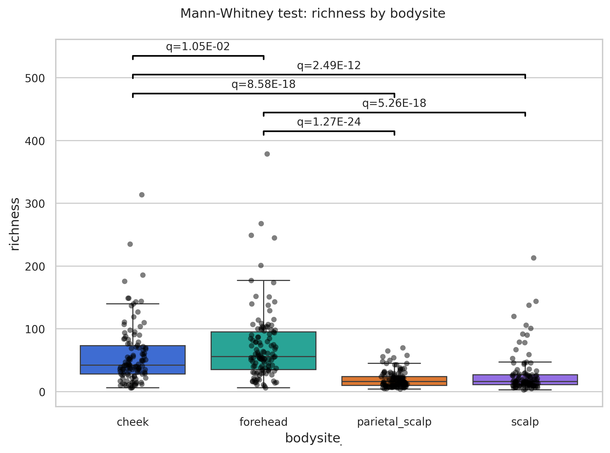
Boxplot of alpha diversity (richness) across skin samples grouped by body site. Each box shows the interquartile range with the median line; whiskers extend to 1.5× IQR, and points beyond them are outliers. Individual samples are overlaid as a jitter plot. Brackets above the boxes display FDR-corrected q-values from pairwise Mann–Whitney U tests between body sites.
- Title: the statistical test, the metric shown, and the grouping variable (for example, Mann-Whitney test: richness by hiv_riskgroup_text).
- Axes: the selected metric on the y-axis; the grouping variable on the x-axis, one boxplot per group.
- Brackets between boxplots: every significant pairwise comparison, labelled with its FDR-adjusted q-value.
The Grouping Variable parameter sets how samples are split into groups along the x-axis: pick the metadata variable whose effect you want to study, such as disease status, treatment, or body site.
The Statistical Test Type sets which test is run between groups. Each selected test runs pairwise on every pair of groups, and a bracket is drawn for a pair when its FDR-adjusted q-value falls below the FDR threshold. You must select at least one, and each selected test produces its own panel.
Which test fits my design?
First ask: are the same subjects measured in more than one group, or are all subjects different?
- Use
Mann–Whitney Ufor independent groups.
Example: You compare alpha diversity between 10 treated mice and 10 untreated mice. Each mouse appears in only one group, so values cannot be paired across groups. The groups are independent →Mann–Whitney Uis appropriate. - Use
Wilcoxonfor paired or matched samples.
Example: You compare alpha diversity in the same 10 mice before and after treatment. Each mouse contributes one “before” and one “after” value, so every value has a natural partner from the same animal. The samples are paired →Wilcoxontests the within-subject change.
Mann–Whitney U is the correct nonparametric test.How Statistical testing works on this module:
Each test you choose from the Statistical Test Type parameter is applied pairwise: it runs on every pair of groups that can possibly be composed from your groups, comparing their alpha diversity distributions two at a time. With three groups, for example, this means three comparisons (A versus B, A versus C, B versus C), whereas four groups means 6 comparisons, and 8 groups means 28.More comparisons means more hypotheses tested, something that inflates the chance of false positives, results that by chance fall below the significance threshold even when the two groups are truly equal.This is the multiple comparisons problem. For this reason, the list of p-values for all the comparisons must be corrected for multiple testing using FDR (Benjamini-Hochberg), which raises each p-value according to how many comparisons were made, so a difference is called significant only if it would still stand out among that many tests.If a pairwise comparison is still significant after correction (below the FDR threshold), the corrected value, the q-value, is what appears on the bracket.We recommend treating a comparison as statistically significant only when its FDR-adjusted q-value falls below your chosen FDR threshold.
Each test you choose from the Statistical Test Type parameter is applied pairwise: it runs on every pair of groups that can possibly be composed from your groups, comparing their alpha diversity distributions two at a time. With three groups, for example, this means three comparisons (A versus B, A versus C, B versus C), whereas four groups means 6 comparisons, and 8 groups means 28.More comparisons means more hypotheses tested, something that inflates the chance of false positives, results that by chance fall below the significance threshold even when the two groups are truly equal.This is the multiple comparisons problem. For this reason, the list of p-values for all the comparisons must be corrected for multiple testing using FDR (Benjamini-Hochberg), which raises each p-value according to how many comparisons were made, so a difference is called significant only if it would still stand out among that many tests.If a pairwise comparison is still significant after correction (below the FDR threshold), the corrected value, the q-value, is what appears on the bracket.We recommend treating a comparison as statistically significant only when its FDR-adjusted q-value falls below your chosen FDR threshold.
A special statistical test: Kruskal-Wallis and Dunn’s test
Alongside the pairwise tests you select, the module always runs a Kruskal-Wallis test followed by Dunn’s post-hoc test. These answer a different question from your chosen tests, which is why it helps to read them together.- Kruskal-Wallis is a single non-parametric test (it does not assume normal data) that asks one global question: does at least one group differ from the rest? Because it is one test rather than many, its false-positive rate does not grow with the number of groups the way a set of separate pairwise tests does, so it is a useful first check of whether there is any group effect at all. It does not say which groups differ.
- Dunn’s post-hoc test identifies which pairs drive a significant Kruskal-Wallis result. It ranks all samples together and compares each pair using the whole dataset, so its pairwise results stay consistent with the global test and with each other. The false-positive rate across Dunn’s pairs is then held in check by the FDR correction described above, not by Kruskal-Wallis itself.
df_kruskal.csv and df_dunn.csv, included in the output export of the module.
Why is this plot useful?
- Assess the impact of biological factors on within-sample diversity: boxplots sitting at clearly different heights, with a significant bracket, suggest that the biological factor (disease, treatment, diet) might be a driver of community composition and richness.
- Spot outliers within single groups: single dots far from the main distribution might flag a contaminated sample (usually richer, depending on how rich the contamination source is), a mislabelled sample, or a genuine outlier pointing to a distinct responder.
- Which part of the community changed: comparing the richness, Shannon, and Simpson panels shows where the change sits. A difference in richness but not Simpson means rare taxa shifted while the dominant members held steady, pointing to a different mechanism than a change among the dominant community.
- Dose-response trend: when the grouping variable has a natural order, such as disease stage or time after treatment, a stepwise rise or fall across the boxes suggests a monotonic relationship between alpha-diversity and the variable.
Statistical output tables
Export the per-sample alpha-diversity values and the full statistical results of the pairwise comparisons by scrolling to the end of the output page and clicking Download Tables and Images:Recommended parameters
Select your workflow to see the recommended values. Note that pre-processing parameters vary per data type.- Kepler - Host-Agnostic Taxonomic Profiling (WGS)
- CHAMP - Human Taxonomic Profiling (WGS)
- 16S SR Amplicon Classification - Taxonomic
- 16S LR Amplicon profiling - Taxonomic
- Host-Agnostic Functional Profiling (WGS)
- CHAMP - Human Functional Profiling (GBM, GMM, KEGG)
- Kepler (WGS) -AMR/VF
Analysis parameter reference
Grouping Variable
Grouping Variable
The metadata column used to define the groups compared in the analysis. It should reflect the biological question or study hypothesis you want to test.Options · Categorical variables from the metadata table associated with the query used to create the analysisDefault ·
NoneSuggested · A categorical variable relevant to your study design, such as treatment, disease status, condition, body site, cohort, or time point.When no grouping variable is selected, alpha-diversity values are shown for the whole cohort, with no group-based comparison.
Alpha-diversity metric
Alpha-diversity metric
The diversity metric(s) calculated per sample and plotted on the y-axis. You can select more than one; each produces its own set of panels.Options ·
richness, shannon, simpsonStatistical Test Type
Statistical Test Type
The statistical test used to compare alpha-diversity values between groups. Available when a Grouping Variable is selected. The right test depends on your study design, in particular whether samples are independent or paired/matched. In addition to the test(s) you choose here, Kruskal-Wallis (followed by Dunn’s post-hoc) is always run and reported.Options ·
Wilcoxon, Mann-Whitney, T-testWhich test fits my design?
First ask: are the same subjects measured in more than one group, or are all subjects different?
First ask: are the same subjects measured in more than one group, or are all subjects different?
- Use
Mann–Whitney Ufor independent groups.
Example: You compare alpha diversity between 10 treated mice and 10 untreated mice. Each mouse appears in only one group, so values cannot be paired across groups. The groups are independent →Mann–Whitney Uis appropriate. - Use
Wilcoxonfor paired or matched samples.
Example: You compare alpha diversity in the same 10 mice before and after treatment. Each mouse contributes one “before” and one “after” value, so every value has a natural partner from the same animal. The samples are paired →Wilcoxontests the within-subject change.
Mann–Whitney U is the correct nonparametric test.P-value threshold
P-value threshold
The p-value cutoff that controls which pairwise comparisons get a significance bracket on the boxplots. It’s applied to the raw p-value of every pairwise test you selected, in each panel (one panel per alpha-diversity metric), so it governs the significance brackets shown between groups, not which features or metrics are analyzed.Options · Numeric value between
0 and 1Default · 0.05Suggested · Use 0.05 as the standard threshold. A more stringent value such as 0.01 reduces the chance of reporting false positives.This threshold is applied to the original (unadjusted) test p-value. Use the FDR threshold below to gate significance on the multiple-testing-corrected value instead.
FDR threshold
FDR threshold
The threshold used to report significance after multiple-testing correction (Benjamini-Hochberg). This matters most when the grouping variable has many categories: more groups means more pairwise comparisons, and FDR adjustment keeps the overall rate of false positives across all of them in check.Options · Numeric value between
0 and 1Default · 0.05Suggested · Use 0.05 as standard. A more stringent value such as 0.01 gives stronger control over false positives when many comparisons are performed.