

Module output and customization
- Annotated Stacked Bar Chart: a stacked bar chart to inspect and compare microbial composition across your cohort, one bar per sample or per group. Sample metadata can be highlighted above the bars, and samples can be sorted, faceted, or collapsed by your variables of interest.
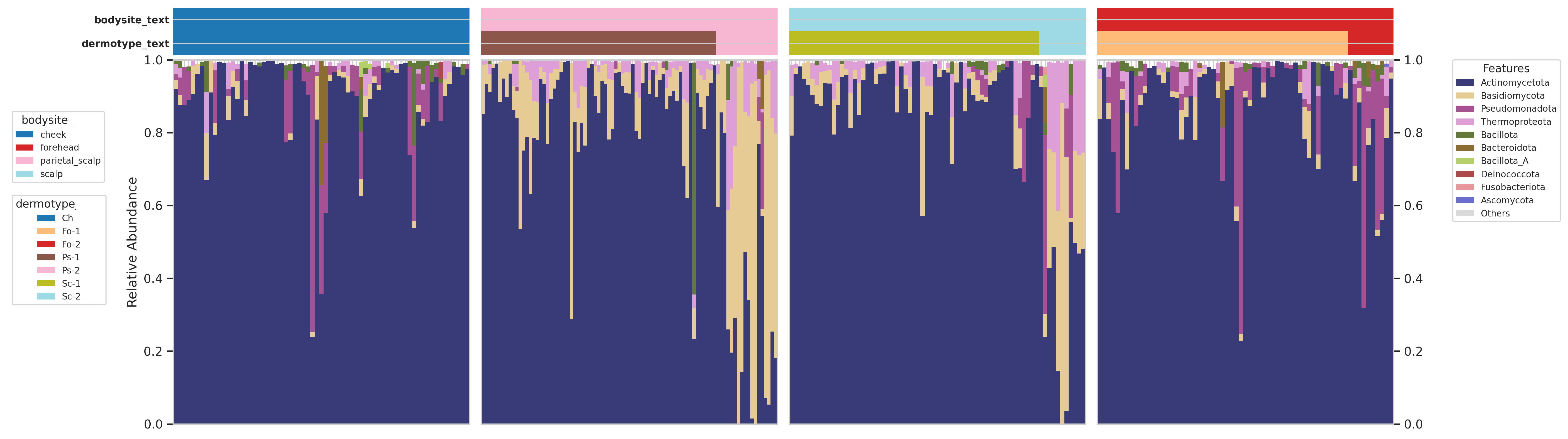
Stacked bar chart of phylum-level relative abundances across skin samples, faceted by body site and sorted by dermotype within each facet. Each bar represents one sample, with segments colored by phylum. Low-abundance phyla are grouped under "Others." Color-coded annotation strips above each facet indicate the body site and dermotype of each sample.
Annotated Stacked Bar Chart
1. Set the bar values and scale
absolute and Analysis Metric to countsrelativeshows the proportion of every feature within the sample. Sample bars reach the same height. Best for comparing composition across samples.absoluteshows feature counts, so bar heights may also reflect differences in sequencing depth or total counts between samples.
2. Choose how features to show per each Bar
The colored segments are the microbial features (taxa or functions). A single sample profile can include hundreds of features (thousands or more for functional profiles), which can make it hard to visualize all of them within the same Bar. To facilitate comparison between samples, it is suggested to limit the number of features shown per bar by visualizing the most abundant, prevalent or variable features across the cohort, and group remaining features into an aggregate category (Others).- Use the Top features (N) parameter to set how many features are displayed individually, and Feature ranking method to decide the ranking criteria to sort microbial features to be selected:
last, since these represent less informative features.
3. Annotate samples with metadata
The colored strips above the bars display sample metadata chosen.- Choose which metadata to display through Sample annotation parameter: categorical variables (sex, treatment, disease status, cohort) appear as distinct colors, and numerical variables (age, BMI) as a continuous scale.
- Remove from the plot samples lacking chosen annotation by checking Drop samples with missing annotation.
4. Set the feature colors
The colors of the feature segments are set by the Feature color palette. Since communities are compared visually by color, a clear, distinguishable palette is what lets real compositional differences stand out rather than blur together among similar shades. This affects appearance only, not the data.5. Arrange and group the samples
How the bars are organized is controlled by Sample arrangement, with three options:Sort uses Sample ordering metadata to set the order, with Samples in ascending order for the direction. This places samples that share a value (same treatment, cohort, or disease status) next to each other. The ordering options come from whatever you selected in Sample annotation.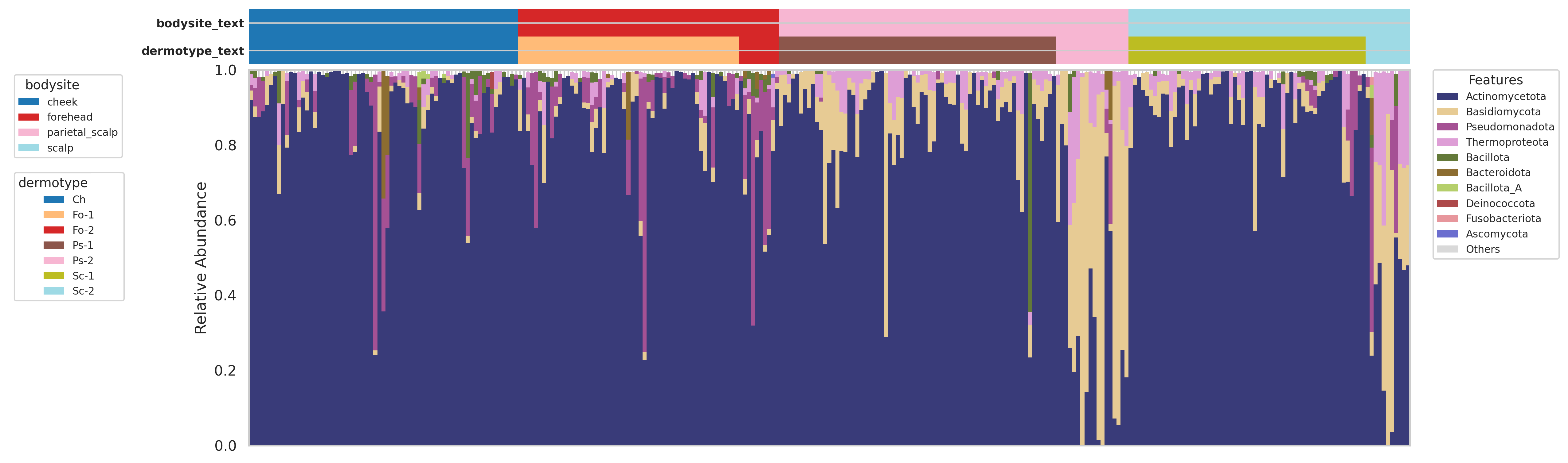
Stacked Bar Chart obtained by setting Sample Arrangement to 'sort', and using 'bodysite ' and 'dermotype' as Sample ordering metadata
Facetalso uses Sample ordering metadata to order samples within each panel, and adds Metadata columns for faceting to choose the variable that splits the panels.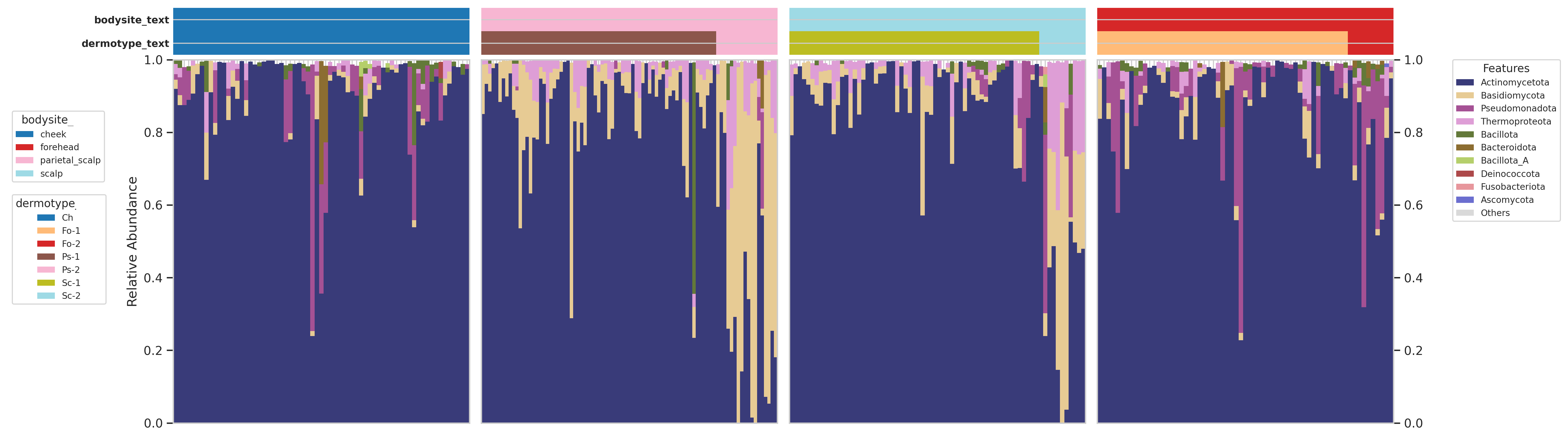
Stacked Bar Chart faceted by Bodysite and sorted by Dermotype
Collapsealso uses Sample ordering metadata to define the groups, and shows one bar per group. Each feature segment is the collapsed (summed) composition of the samples in that group, displayed as relative abundance. This is useful for spotting features that shift on group average, but it hides sample-to-sample variability, so it is best when group-level patterns matter more than individual samples.
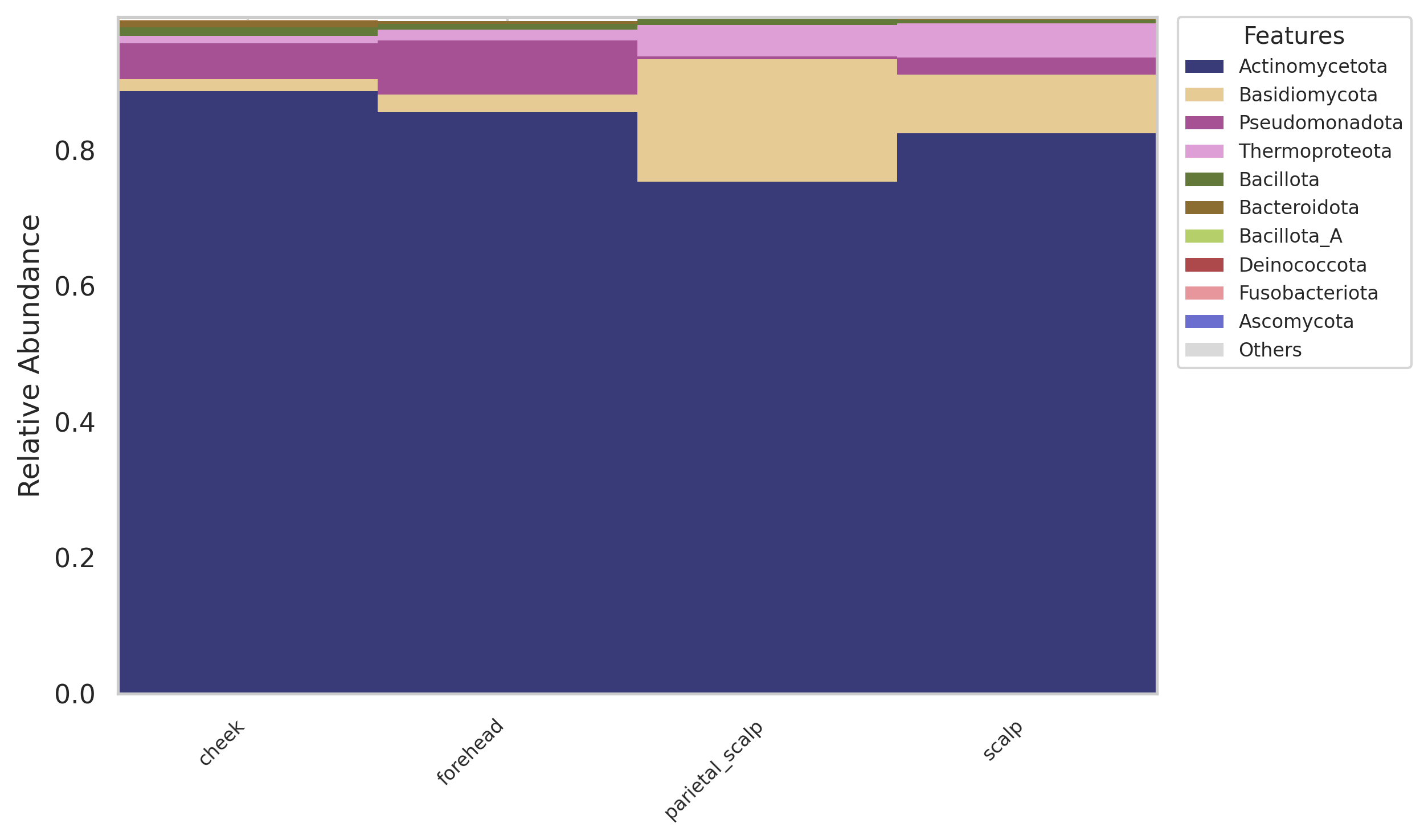
Stacked barchart obtained by setting Sample Arrangement to 'collapse' and 'ethnicity' as Sample Ordering Metadata
Sort, Facet, and Collapse all reveal Sample ordering metadata (and its direction). Facet additionally reveals Metadata columns for faceting. In every case, the metadata available for ordering is whatever you chose in Sample annotation.6. Show or hide sample labels
Show sample labels toggles the sample names along the x-axis. Keep them on for small cohorts where identifying individual samples helps, and off for large cohorts where labels would crowd the plot.Recommended parameters
Pre-processing
Select your workflow. These pre-processing values vary by data type; the display settings below are the same regardless of workflow.- Kepler - Host-Agnostic Taxonomic Profiling (WGS)
- CHAMP - Human Taxonomic Profiling (WGS)
- 16S SR Amplicon Classification - Taxonomic
- 16S LR Amplicon profiling - Taxonomic
- Host-Agnostic Functional Profiling (WGS)
- CHAMP Functional (GMM, GBM, KEGG)
- AMR/VF - Functional
Stacked Bar Chart settings
Parameter reference
Sample Annotation
Sample Annotation
NoneSuggested · Variables relevant to the biological question, such as treatment, disease status, body site, cohort, time point, age group, sex, or sequencing batch. Avoid selecting too many, or the plot becomes hard to read.Drop samples with missing annotation
Drop samples with missing annotation
TRUE (drop them) or FALSE (keep them)Default · TRUESuggested · Leave TRUE when the annotation is essential and unannotated samples should not appear. Use FALSE to preserve sample size and see where unannotated samples fall.TRUE, samples missing the chosen annotation are removed from the plot. When FALSE, they are kept and assigned to a default missing-value group.Feature Ranking Method
Feature Ranking Method
mean, prevalence, variance, percentileDefault · meanSuggested · percentile is balanced, surfacing features that reach high abundance in a meaningful fraction of samples. Use mean for dominant features, prevalence for widely shared ones, and variance for features that change strongly across samples.percentile ranks each feature by the 90th percentile of its abundance across samples (zeros included), so sparse features that spike in only a few samples still rank low. Different methods surface different biological patterns.Top Features (N)
Top Features (N)
1 to 30 Default · 10Suggested · 5–20 depending on dataset complexity and readability; 10 is a practical default.N are displayed individually; the rest are grouped into Others / Unassigned. For example, mean ranking with N = 10 shows the 10 features with the highest average abundance.Y-axis Values
Y-axis Values
absolute, relativeDefault · absoluteSuggested · relative for most cross-sample comparisons, since it makes bars directly comparable. absolute when read-count differences are biologically or technically relevant.Feature Color Palette
Feature Color Palette
tab20bSuggested · A palette that makes features easy to tell apart. Discrete palettes are recommended, since each color represents a different taxon or function.Show Sample Labels
Show Sample Labels
TRUE or FALSEDefault · TRUESuggested · TRUE for small cohorts where identifying samples helps; FALSE for many samples where labels crowd the plot.Sample Arrangement
Sample Arrangement
None, sort, facet, collapseDefault · None (samples are ordered alphabetically by sample name)Suggested ·None, no metadata ordering; samples are ordered alphabetically by sample name.sort, order samples by metadata so similar samples sit together.facet, split into panels by a categorical variable to compare groups while keeping individual bars.collapse, summarize into group-level bars for a compact overview.
sort, facet, and collapse all enable Sample ordering metadata, and facet additionally enables Metadata columns for faceting. Example: to compare taxonomic profiles across cancer subtypes while showing treatment status, facet by subtype and annotate by treatment.Sample Ordering Metadata
Sample Ordering Metadata
sort, facet, or collapse.The metadata column(s) used to order samples. The available choices are the variables you selected in Sample annotation.Options · Any metadata chosen in Sample annotationDefault · NoneSuggested · A variable that makes the plot easier to read, such as disease status, treatment, cohort, time point, body site, or read depth. Sorting by read depth, for instance, can reveal whether composition tracks sequencing depth.Samples in Ascending Order
Samples in Ascending Order
TRUE (ascending) or FALSE (descending)Default · TRUESuggested · Whichever direction makes the plot easiest to interpret. Affects visual order only, not feature values or sample inclusion.Place "Others" / "Unassigned"
Place "Others" / "Unassigned"
Others / Unassigned segment, which combines the abundance of all features outside the top N, appears at the top or the bottom of each sample’s bar.Options · first, lastDefault · lastSuggested · last for most plots, since this segment represents aggregated, less informative features.N are grouped into Others / Unassigned to keep the chart readable; this controls where that group sits in the bar.Metadata Columns for Faceting
Metadata Columns for Faceting
facet.The categorical column used to create panels when the chart is faceted.Options · Categorical columns chosen in Sample ordering metadataDefault · NoneSuggested · A categorical variable defining the main groups to divide the chart into, such as disease status, treatment, cohort, body site, cancer subtype, or time point.facet. Example: faceting by cancer subtype creates a panel per subtype, while sample annotations can still show treatment, sex, or cohort.