

Module output and customization
- Feature-level group comparison boxplot panels: One panel for each differentially abundant feature, repeated for each abundance test you selected. Within a panel, one boxplot per group shows how that feature’s relative abundance is distributed across groups of interest.
- Differential prevalence table [1]: A table reporting which features are differentially prevalent (detected in a different proportion of samples) across your groups of interest.
- Univariate Statistical testing tables [3]: Three tables reporting the statistical output for the abundance and prevalence test: the Kruskal-Wallis test per feature (always run), the Dunn’s post-hoc pairwise comparisons, and the pairwise differential-abundance results from your selected test.
Feature-level group comparison boxplot panels
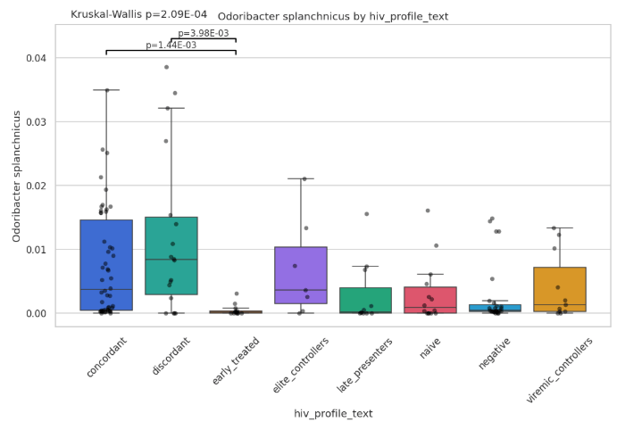
Feature-level group comparison. The distribution of one feature across groups, one dot per sample. Brackets mark significant pairwise comparisons; the title reports the overall group-level test.
Define which groups to compare
Univariate comparison finds which microbial features are associated with a categorical variable of interest by testing which features are differentially abundant or prevalent between its groups. Select one categorical metadata variable using the Grouping Variable parameter. The values of this variable define the groups that every feature is compared across.Choosing the right statistical test for group comparison
Univariate Comparison module find abundance and prevalence associations to your variable of interest by running statistical tests on all possible pairwise group combinations. Depending on this, choose which tests you want to use: Differential abundance compares the relative abundance of each feature between groups. Use the Differential Abundance test dropdown to choose which statistical test is used for testing differential abundances:Mann-Whitney Ufor independent groups (e.g: cross-sectional unrelated subjects)Wilcoxon signed-rankfor paired samples (e.g: subjects longitudinally sampled)t-testwhen comparing distributions that are approximately normal.
Which test fits my design?
First ask: are the same subjects measured in more than one group, or are all subjects different?
- Use
Mann–Whitney Ufor independent groups.
Example: You compare alpha diversity between 10 treated mice and 10 untreated mice. Each mouse appears in only one group, so values cannot be paired across groups. The groups are independent →Mann–Whitney Uis appropriate. - Use
Wilcoxonfor paired or matched samples.
Example: You compare alpha diversity in the same 10 mice before and after treatment. Each mouse contributes one “before” and one “after” value, so every value has a natural partner from the same animal. The samples are paired →Wilcoxontests the within-subject change.
Fisher's exactthe standard, conservative default. Fast and reliable, especially with small samples.Barnardmore powerful than Fisher for two-group comparisons, but computationally heavy and might require more time to run.Boschlooat least as powerful as Fisher for two-group comparisons. Choose it when sensitivity matters most.
Kruskal-Wallis + Dunn testAlongside your chosen test, a Kruskal-Wallis test with Dunn’s post-hoc always runs. Kruskal-Wallis is a non-parametric test that asks whether a feature’s distribution differs across all groups at once, and Dunn’s post-hoc then identifies which specific group pairs differ. The same logic appears in the alpha diversity group comparisons.
Choose when a feature association counts as significant
Significance brackets and p-values/q-values of boxplot panels are reported when comparisons are reported as statistically significant. Choose statistical significance threshold (usually 0.05) through P-value threshold parameter. Because many features and group pairs are tested at once, the risk of incurring in associations that are false positives increases significantly. This is why p-values are usually adjusted (Q-value) by weighting on how many hypotheses have been tested. Set the False Discovery Rate threshold to decide when a Q-value should be marked as significant.- Diff. Abundance tests FDR threshold for the abundance comparisons between more than
- Diff. Prevalence tests FDR threshold for the prevalence comparisons.
Note: a boxplot panel of a feature is displayed only when there’s at least a pair of groups where the differentially abundant feature association was found to be statistically significant.Deciding where to set this threshold depends on the goals of the analysis and how confident you need to be. To produce plots also for exploratory purposes and see feature-level group boxplots panels for features that we suggest to increase the FDR threshold
The P-value threshold is a fallback, not the main cutoff. When a run has too few tests for multiple-testing correction to be meaningful (for example, only one valid comparison for a test), significance falls back to this raw p-value threshold instead of the FDR one. In a normal multi-taxon run, the two FDR thresholds are what matter.
Set how many panels are shown
A real dataset can produce more significant features than are useful to view at once.- The Max figures to display parameter limits how many boxplots appear on screen per test, showing only the top results. Note that exporting includes every significant feature’s boxplot, not just those shown on screen.
Why is this plot useful?
- Reveals associations between a feature and a clinical or experimental variable. It tells you whether a taxon’s abundance is statistically associated with the grouping variable, which is a starting point for relating that microbe to disease, treatment, or other characteristics.
- Localizes the association to specific groups. The pairwise comparisons show which groups a feature distinguishes, pinpointing where the association is strongest.
- Separates statistical significance from biological size. Showing the full distribution alongside the p-values lets you judge whether a significant association is also a sizeable, consistent shift, rather than a small difference made significant by sample size.
- Generates focused, testable hypotheses. Out of thousands of features, it isolates one feature and a specific set of group differences as candidate markers for follow-up.
Univariate Statistical Testing tables
- Contingency Tests
- Kruskal–Wallis
- Dunn's Post-hoc
- Diff. Abundance Pairwise
Prevalence testing asks whether a feature is detected in a different proportion of samples across groups, rather than whether its amount differs. For each feature, the number of samples where it is present and absent is tabulated per group, and the contingency test you selected in Differential Prevalence Test evaluates whether detection frequency differs more than chance would explain. The results are FDR-corrected using the Diff. Prevalence tests FDR threshold.
Recommended parameters
Select your workflow. Read depth recommendations and supported pre-processing methods differ by data type; the analysis parameters are otherwise consistent.- Kepler - Host-Agnostic Taxonomic Profiling (WGS)
- CHAMP - Human Taxonomic Profiling (WGS)
- 16S SR Amplicon Classification - Taxonomic
- 16S LR Amplicon profiling - Taxonomic
- Host-Agnostic Functional Profiling (WGS)
- CHAMP Functional (GMM, GBM, KEGG)
- AMR/VF - Functional
Parameter reference
Grouping Variable
Grouping Variable
The metadata column that defines the groups to compare. This is the comparison the whole module performs.Options · Categorical variables from the metadata table associated with the query used to create the analysisDefault ·
NoneSuggested · A categorical variable reflecting your biological question, such as disease status, treatment, response status, body site, cohort, time point, or HIV profile.Drop samples with missing grouping metadata
Drop samples with missing grouping metadata
Whether samples with missing values in the grouping variable are removed from the analysis.Options ·
TRUE or FALSEDefault · TRUE Differential Prevalence Test
Differential Prevalence Test
One or more tests comparing feature prevalence (how often a feature is detected) across groups.Options ·
fisher, barnard, boschlooDefault · fisherDifferential Prevalence Tests FDR Threshold
Differential Prevalence Tests FDR Threshold
The FDR threshold for reporting significant differential-prevalence results after p-value adjustment.Options ·
0.01 to 1.0, step 0.01Default · 0.1Differential Abundance Test
Differential Abundance Test
The statistical test used to compare alpha-diversity values between groups. Available when a Grouping Variable is selected. The right test depends on your study design, in particular whether samples are independent or paired/matched. In addition to the test(s) you choose here, Kruskal-Wallis (followed by Dunn’s post-hoc) is always run and reported.Options ·
Wilcoxon, Mann-Whitney, T-testWhich test fits my design?
First ask: are the same subjects measured in more than one group, or are all subjects different?
First ask: are the same subjects measured in more than one group, or are all subjects different?
- Use
Mann–Whitney Ufor independent groups.
Example: You compare alpha diversity between 10 treated mice and 10 untreated mice. Each mouse appears in only one group, so values cannot be paired across groups. The groups are independent →Mann–Whitney Uis appropriate. - Use
Wilcoxonfor paired or matched samples.
Example: You compare alpha diversity in the same 10 mice before and after treatment. Each mouse contributes one “before” and one “after” value, so every value has a natural partner from the same animal. The samples are paired →Wilcoxontests the within-subject change.
Mann–Whitney U is the correct nonparametric test.Differential Abundance Tests FDR Threshold
Differential Abundance Tests FDR Threshold
The FDR threshold for reporting significant differential-abundance results after p-value adjustment.Options ·
0.01 to 1.0, step 0.01Default · 0.1Suggested · 0.05 for standard analyses; 0.1 for exploratory or small studies; lower for high-dimensional or confirmatory analyses.Applied after multiple-testing correction. Lower values give a shorter, more conservative list; higher values increase sensitivity and false positives.
P-value Threshold
P-value Threshold
A fallback significance cutoff, applied only when there are too few tests for multiple-testing correction to be meaningful. In normal runs, significance is shown as the FDR thresholds instead, so this parameter usually has no effect.Options ·
0.01 to 1.0, step 0.01Default · 0.05Max Figures to Display
Max Figures to Display
The maximum number of feature-level boxplots shown on screen per test.Options ·
0 to 20, step 1Default · 5Suggested · 5 for a concise output; 10–20 to inspect more significant results in the interface.