16S Metagenomics Profilng Methodology
Within DADA2, forward and reverse reads are each trimmed to a uniform length based on the quality of reads in the sample—higher quality data will generally result in longer reads. DADA2 uses machine learning with a parametric error model to learn the error rates for the forward and reverse reads, based on the premise that correct sequences should be more common than any particular error-variant. DADA2 then applies its core sample inference algorithm to the filtered and trimmed data, applying these learned error models. Paired-end reads are then merged if they have at least 12 bases of overlap and are identical across the entire overlap. The resulting table of sequences and observed frequencies is filtered to remove chimeric sequences (those that exactly match a combination of more-prevalent “parent” sequences). Taxonomy and species-level identification (where possible) are conducted with DADA2’s naive Bayesian classifier, using the Silva version 138 database. Lastly, the predicted functional potential of the community was profiled using PICRUST2 (5)(6)(7)(8)(9). Briefly, PICRUSt2 (Phylogenetic Investigation of Communities by Reconstruction of Unobserved States) is a tool that predicts functional capabilities and abundances of a microbial community based on the observed amplicon (marker gene) content. Functional capabilities are given by EC classifiers, or MetaCyc ontologies, and these can be aggregated to predict pathways that are likely present in a given sample.What is a primer sequence and why is it needed to for 16S workflow?
Primers are short, artificial DNA strands of about 18 to 25 nucleotides that match the beginning and end of the DNA fragment to be amplified. In amplicon sequencing methods, PCR with specific primers produces the amplicon of interest. These primer sequences need to be trimmed from the reads before further processing and any downstream analytics. Please do not use any technical sequence such as adapter sequences but only the primer sequence that matches the biological amplicon. For example: —Forward Primer “GTGYCAGCMGCCGCGGTAA” —Reverse Primer “GGACTACNVGGGTWTCTAAT”What does the different modes (Mode Q25, Q20 and Q15) represent for Amplicon 16S results view?
The modes Q15, Q20, and Q25 represent distinct Phred quality score thresholds utilized in the Amplicon 16S workflow. For example, mode Q25, with a Phred quality score of 25, ensures that retained reads maintain a median quality score of 25 across the read’s length, along with a maximum expected error of 6 bases per read. Moreover, for each mode, a minimum of 20% of reads per sample will be preserved. However, if there are insufficient reads meeting the respective Phred score quality thresholds, the results will progressively incorporate lower quality reads to achieve the minimum requirement.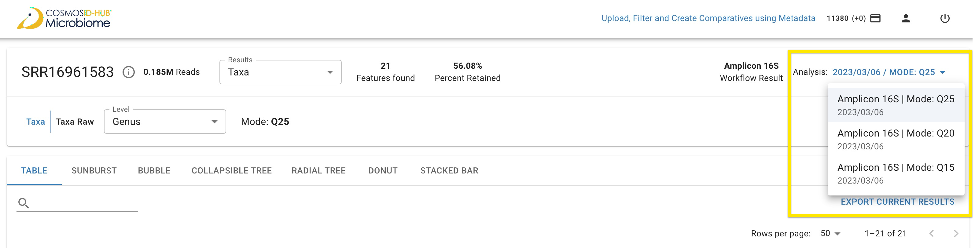
What is an ASV?
An amplicon sequence variant (ASV) is any one of the inferred single DNA sequences recovered from a high-throughput sequencing analysis of marker genes. Because these sequences are created following the removal of erroneous sequences generated during PCR and sequencing, using ASVs makes it possible to distinguish sequence variation by a single nucleotide change. The uses of ASVs include classifying groups of species based on DNA sequences, finding biological and environmental variation, and determining ecological patterns.What does the “ASV count” represent on the single sample taxonomic results explorer?
The ASV count represents the number of observations of an ASV in that sample.What does the “raw count” represent on the single sample functional results explorer?
The raw count represents the read depth per ASV multiplied by the predicted function abundances per ASV.Why would you choose ASVs methods over OTUs methods for inferring taxonomic composition from your 16S data?
OTU clustering reduces resolution by clustering similar sequences over a certain threshold into one specific sequence or one specific consensus sequence. ASVs capture the fine scale variation that exists and allows more sensitivity and thus the ability to get closer to “True” taxonomic compositionThe advantages of ASVs over OTUs
- There are many arguments in the microbiome community to move 16S analysis approach to ASV based methods (10)
- ASV methodology have showcased sensitivity and specificity as good or better than OTU methods and allow better discrimination of ecological patterns (10)
- ASV methods are reproducible since these are exact sequences, generated without clustering or reference databases (10)
- OTUs often overestimate bacterial richness when compared to ASVs (10)
What does the “percentage of reads retained” imply?
You can track how many reads were retained and rejected through each step in the 16S workflow. It’s normal to lose some reads during each step, but large drops at particular steps can indicate specific issues with the data. For example, if a large number of reads are lost during filtering, it could indicate poor sequence data overall, while a major decrease at the chimera-removal step frequently indicates an issue with primer removal, so we suggest confirming the primer sequences are correct and adapters are trimmed.How do you upload your 16S amplicon data to the HUB?
You have the option to upload your data from your desktop or your Illumina BaseSpace account or from NCBI SRA as well.How do you generate comparative analysis to aggregate and compare your 16S results across cohorts?
Results can be downloaded or compared to other 16S samples for visualizations through the Cosmos-Hub Comparative Analysis tool. 16S OTU Workflow Methodology For taxonomic profiling based amplicon 16S data, the Cosmos-Hub 16S data analysis pipeline starts with preprocessing of the raw reads from either paired-end or single-end Fastq files through read-trimming to remove adapters as well as reads and bases of low quality. If the reads are in a paired-end format, the forward and reverse overlapping pairs are joined together; the unjoined R1 and R2 reads are then added to the end of the file. The file is then converted to Fasta format and used as input for OTU picking. OTUs are identified against the Cosmos-Hub curated 16S database using a closed-reference OTU picker and 97% sequence similarity through the QIIME framework. The final results are then presented in tabular format with the taxonomic names, OTU IDs, frequency, and relative abundance. Results can be downloaded or compared to other 16S samples for visualizations through the Cosmos-Hub Comparative Analysis tool.Why Are Mitochondria and Chloroplasts Showing Up in My 16S Data?
It’s common for researchers to observe mitochondrial and chloroplast reads in their 16S rRNA sequencing results—especially when analyzing samples derived from plant or eukaryotic tissue (e.g., roots, leaves, gut biopsies). This is not an error or contamination in the workflow, but rather a well-understood and expected limitation of current 16S sequencing approaches and reference databases.The Evolutionary Origin: Why This Happens
Mitochondria and chloroplasts are endosymbiotic organelles that originated from free-living bacteria. As such, they retain genes, including the 16S rRNA gene, that are evolutionarily and structurally homologous to bacterial 16S genes. Even though most 16S protocols use bacterial-specific primers (e.g., V3–V4 or V4), these primers can still amplify organellar 16S genes due to sequence similarity. This leads to co-amplification of host-derived (eukaryotic) sequences, particularly:- Mitochondrial 16S rRNA, typically from animal tissue in gut or fecal samples
- Chloroplast 16S rRNA, highly abundant in plant material such as root or leaf tissues, or soil containing plant detritus
A Database-Level Constraint
The Cosmos-Hub platform uses the SILVA 16S rRNA gene reference database, a gold-standard, curated, and taxonomically comprehensive resource. Importantly, SILVA includes mitochondrial and chloroplast sequences as part of its taxonomy structure. As a result, if those sequences are present in the input FASTQ files, they will be profiled alongside true bacterial sequences. This is a standardized behavior across all tools using SILVA (or similarly broad 16S databases) and is not specific to Cosmos-Hub.How to Address This
Because mitochondrial and chloroplast sequences are legitimate reads from the sample’s DNA content, they cannot be filtered after taxonomic profiling has been completed. Instead, the appropriate approach is to remove these reads prior to uploading data into Cosmos-Hub. This is typically done by:- Aligning raw reads against curated mitochondrial and chloroplast databases (e.g., using BLAST, Bowtie2, or BWA).
- Filtering out mapped reads, leaving only bacterial-origin reads.
- Re-processing the filtered FASTQ files through Cosmos-Hub for taxonomic profiling.
Need Help Removing Host-Derived Reads?
The Cmbio team offers custom bioinformatics support for projects requiring removal of organellar reads, especially in plant-rich or host-associated datasets. We typically extract, filter, and clean these reads in a reproducible manner, followed by reprofiling in the Hub. If you’d like us to assist with this as part of your project scope, please contact us directly to initiate a custom analysis plan.References:
- Straub, D. et al. Interpretations of Environmental Microbial Community Studies Are Biased by the Selected 16S rRNA (Gene) Amplicon Sequencing Pipeline. Front. Microbiol. 11, 1–18 (2020).
- Callahan, B. J., McMurdie, P. J. & Holmes, S. P. Exact sequence variants should replace operational taxonomic units in marker-gene data analysis. ISME J. 11, 2639–2643 (2017).
- Callahan, B. J. et al. DADA2: High-resolution sample inference from Illumina amplicon data. Nat. Methods 13, 581–583 (2016).
- Martin, M. Cutadapt removes adapter sequences from high-throughput sequencing reads. EMBnet.journal 17, 10 (2011).
- Douglas, G. M. et al. PICRUSt2 for prediction of metagenome functions. Nat. Biotechnol. 38, 685–688 (2020).
- Barbera, P. et al. EPA-ng: Massively Parallel Evolutionary Placement of Genetic Sequences. Syst. Biol. 68, 365–369 (2019).
- Czech, L., Barbera, P. & Stamatakis, A. Genesis and Gappa: processing, analyzing and visualizing phylogenetic (placement) data. Bioinformatics 36, 3263–3265 (2020).
- MIRARAB, S., NGUYEN, N. & WARNOW, T. SEPP: SATé-Enabled Phylogenetic Placement. in Biocomputing 2012 247–258 (WORLD SCIENTIFIC, 2011). doi:10.1142/9789814366496_0024.
- Louca, S. & Doebeli, M. Efficient comparative phylogenetics on large trees. Bioinformatics 34, 1053–1055 (2018).
- Ye, Y. & Doak, T. G. A Parsimony Approach to Biological Pathway Reconstruction/Inference for Genomes and Metagenomes. PLoS Comput. Biol. 5, e1000465 (2009).
- Chiarello, M., McCauley, M., Villéger, S. & Jackson, C. R. Ranking the biases: The choice of OTUs vs. ASVs in 16S rRNA amplicon data analysis has stronger effects on diversity measures than rarefaction and OTU identity threshold. PLoS One 17, 1–19 (2022).